Stroke Prediction - Cluster Analysis and Dimensionality Reduction
This analysis aimed to enhance stroke data classification models by integrating unsupervised learning techniques like clustering and dimensionality reduction. By employing clustering, we segmented patients into groups with similar features to improve stroke risk classification, and applied dimensionality reduction to explore patterns in the data. Despite the dataset's imbalance, we observed that cluster-based classification could slightly improve results. Specifically, clustering approaches like DBSCAN Clustering, combined with classification algorithms, showed potential in better identifying stroke risk while balancing accuracy and recall. The ultimate goal is to provide early identification of high-risk individuals, optimize resource allocation, and support targeted preventive measures.
1. Main Objective
The main objective of this analysis is to improve derived base classification models of the Stroke Data Analysis by applying unsupervised learning methods like clustering and dimensionality reduction. With clustering we will analyze the data and aim to segment the population into groups of patients with similar features to support classification of stroke risk. Dimensionality reduction aims at transforming the observations in a different space to see whether we can identify some structure or patterns. The metrics for finding the best prediction is again to maximize accuracy in terms of recall whilst not classifying too many cases wrongly as stroke risk. The true cost of misclassifying a patient at stroke risk as healthy outweighs the cost of misclassifying a healthy patient as at risk for stroke. The analysis aims at improving basic classification models and providing further insights for stroke risk to allow:
- Early Identification: Helping healthcare providers identify individuals at higher risk of stroke for timely intervention.
- Resource Allocation: Assisting in the efficient allocation of medical resources to those most in need.
- Preventive Measures: Providing insights for developing targeted preventive measures to reduce the incidence of strokes.
2. Dataset Description
The Stroke Prediction dataset is available at Kaggle (URL : https://www.kaggle.com/fedesoriano/stroke-prediction-dataset) and contains data on patients, including their medical and demographic attributes.
Attributes
| Attribute | Description |
|---|---|
| id | Unique identifier for each patient. |
| gender | Gender of the patient (Male, Female, Other). |
| age | Age of the patient. |
| hypertension | Whether the patient has hypertension (0: No, 1: Yes). |
| heart_disease | Whether the patient has heart disease (0: No, 1: Yes). |
| ever_married | Marital status of the patient (No, Yes). |
| work_type | Type of occupation (children, Govt_job, Never_worked, Private, Self-employed). |
| residence_type | Type of residence (Rural, Urban). |
| avg_glucose_level | Average glucose level in the blood. |
| bmi | Body mass index. |
| smoking_status | Smoking status (formerly smoked, never smoked, smokes, Unknown). |
| stroke | Target variable indicating whether the patient had a stroke (0: No, 1: Yes). |
- Number of Instances: 5,110
- Number of Features: 11
- Target Variable:
stroke(0: No Stroke, 1: Stroke)
Analysis Objectives
The analysis aims to:
-
Explore and visualize the data to understand the distribution of attributes and identify any missing or anomalous values.
-
Engineer features and prepare data.
-
Train multiple clustering models on the new engineered dataset and evaluate the performance of classification based on the clusters.
-
Train multiple dimensionality reduction models and evaluate the performance of classification based on the transformed data.
-
Identify the best-performing model and Feature engineering approach.
-
Provide recommendations for next steps and further optimization.
3. Data Exploration and Cleaning
Data Exploration
Besides the id the dataset includes ten features as listed above plus the target variable stroke . There are three numerical features: age, avg_glucose_level and bmi. The remaining seven features are all categorical.
Out of the 5,110 observations in the dataset, 4861 were observed with no stroke and 249 patients had a stroke. The dataset could be classified as not balanced, which has to be addressed before model training.
The variables of the dataset are shown below.
| count | unique | top | freq | mean | std | min | 25% | 50% | 75% | max | |
|---|---|---|---|---|---|---|---|---|---|---|---|
| gender | 5110 | 3 | Female | 2994 | NaN | NaN | NaN | NaN | NaN | NaN | NaN |
| age | 5110.0 | NaN | NaN | NaN | 43.23 | 22.61 | 0.08 | 25.0 | 45.0 | 61.0 | 82.0 |
| hypertension | 5110.0 | NaN | NaN | NaN | 0.1 | 0.3 | 0.0 | 0.0 | 0.0 | 0.0 | 1.0 |
| heart_disease | 5110.0 | NaN | NaN | NaN | 0.05 | 0.23 | 0.0 | 0.0 | 0.0 | 0.0 | 1.0 |
| ever_married | 5110 | 2 | Yes | 3353 | NaN | NaN | NaN | NaN | NaN | NaN | NaN |
| work_type | 5110 | 5 | Private | 2925 | NaN | NaN | NaN | NaN | NaN | NaN | NaN |
| Residence_type | 5110 | 2 | Urban | 2596 | NaN | NaN | NaN | NaN | NaN | NaN | NaN |
| avg_glucose_level | 5110.0 | NaN | NaN | NaN | 106.15 | 45.28 | 55.12 | 77.24 | 91.88 | 114.09 | 271.74 |
| bmi | 4909.0 | NaN | NaN | NaN | 28.89 | 7.85 | 10.3 | 23.5 | 28.1 | 33.1 | 97.6 |
| smoking_status | 5110 | 4 | never smoked | 1892 | NaN | NaN | NaN | NaN | NaN | NaN | NaN |
| stroke | 5110.0 | NaN | NaN | NaN | 0.05 | 0.22 | 0.0 | 0.0 | 0.0 | 0.0 | 1.0 |
To analyze distribution and correlation of the data we prepared a set of 4 plots for each of the variables despending on the type as follows:
-
Numerical Variables: The overall distribution of the variable, the distribution of the variable for non stroke observations, the distribution of the variable for stroke observations and the density distribution separated by stroke cases.
-
Categorical Variables: The overall distribution of the variable, the distribution of the variable for non stroke observations, the distribution of the variable for stroke observations and the distribution of stroke cases within the groups of the categorical variable.
Numerical Variables
The graphs for the three numerical variables are shown below. There isn't a meaningful correlation visible for BMI or the Average Glucose Level. In contrast Age shows a fairly strong dependency with the target variable.
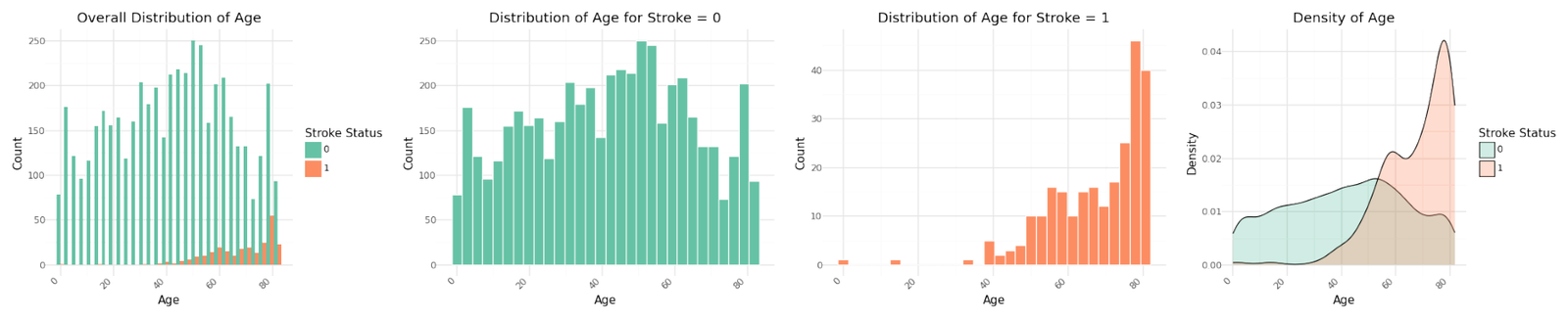
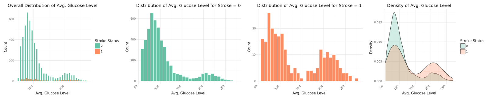
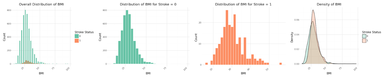
Distribution of numerical variables
Stroke cases plotted versus Age show to be not equally distributed. The reported stroke cases can be more often found with increasing age. Body Mass Index and Average Glucose level do not show an obvious influence on stroke. The observation is confirmed in the pairplot below.
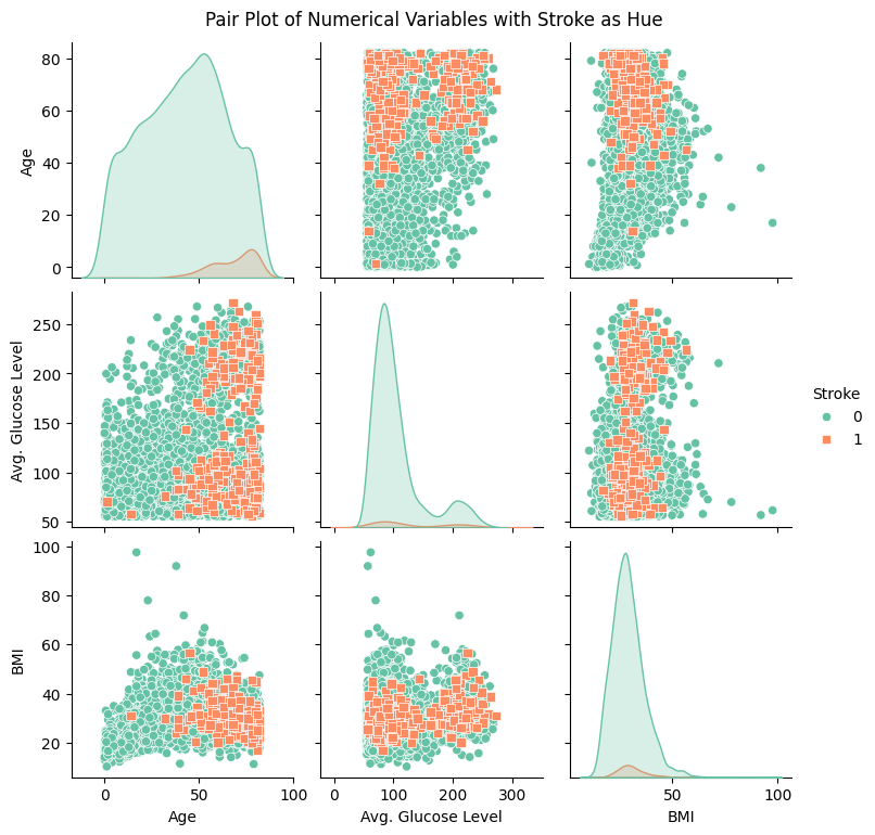
Correlation of numerical variables
Categorical Variables
The graphs for the seven categorical variables are shown below. There isn't a meaningful correlation visible for BMI or the Average Glucose Level. In contrast Age shows a fairly strong dependency with the target variable.
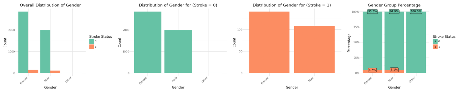
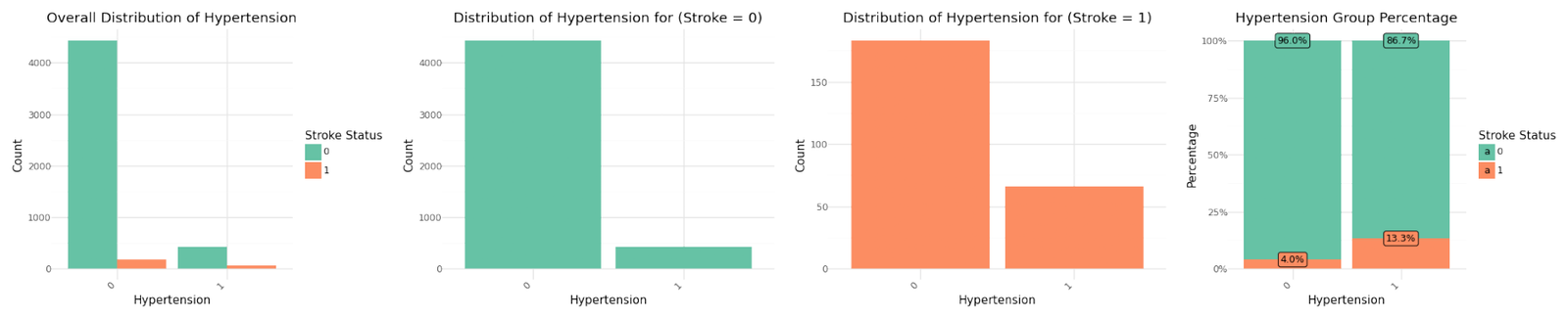

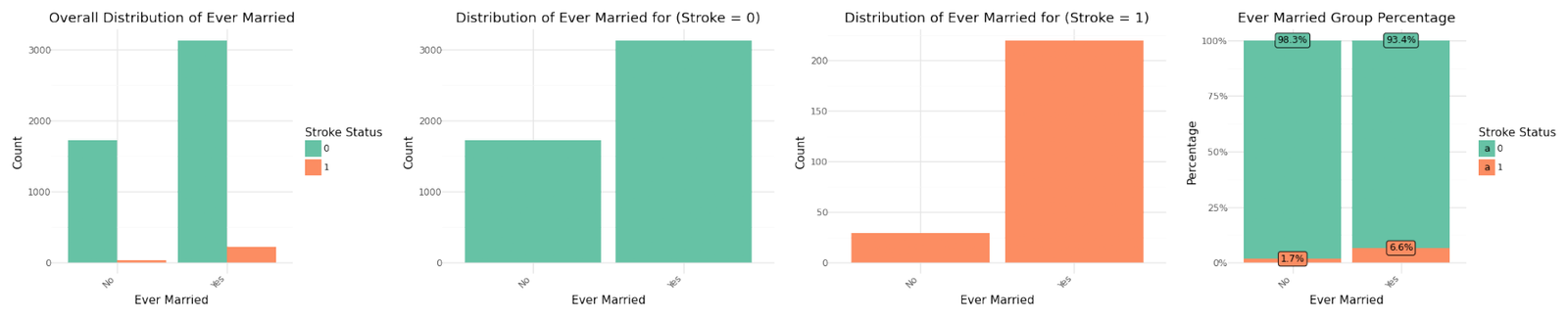
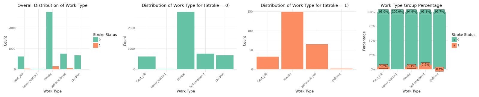
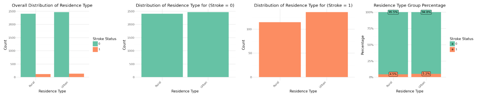
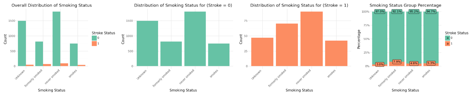
Distribution of categorical variables
If we analyze the group percentages and compare the distributions of the variables for stroke and non stroke cases we can identify Hypertension, Heat Disease and the Married Status as potential influence for stroke cases. We refer to further correlation analysis in Part 1.
Data Cleaning and Feature Engineering
To prepare the data for the further analysis and the modeling phase we will perform the following steps:
- Handling Missing Values and Outliers: Address missing values as appropriate.
- Encoding Categorical Variables: Convert categorical variables into numerical format using one-hot encoding.
- Data Splitting: Split the data into training and testing sets.
- Feature Scaling: Scale features to ensure they are on a similar scale.
- Addressing unbalanced data: Balances the classes in the training set.
Handling Missing Values and outliers
There are 201 records with missing BMI value, from these 201 a count of 40 are stroke cases (Stroke =1). We will adjust the missing values by calculating the group mean BMI by gender, age and glucose level. Further we have to address two outlier stroke cases as well as some more unrealistic BMI outliers.
There are two stroke cases in very early years which can be regarded as outlier. These cases are rather caused by very rare circumstances and should not be part of a systemic data analysis. We drop the records with id 69768 and 49669.
| 162 | 245 | |
|---|---|---|
| id | 69768 | 49669 |
| gender | Female | Female |
| age | 1.32 | 14.0 |
| hypertension | 0 | 0 |
| heart_disease | 0 | 0 |
| ever_married | No | No |
| work_type | children | children |
| Residence_type | Urban | Rural |
| avg_glucose_level | 70.37 | 57.93 |
| bmi | NaN | 30.9 |
| smoking_status | Unknown | Unknown |
| stroke | 1 | 1 |
We also will drop some unrealistic BMI (Body Mass Index) records. A BMI over 70 is extremely high and generally not realistic for most individuals. BMI is calculated as weight in kg divided by height in meter squared For context, a BMI between 18.5 and 24.9 is considered normal weight, a BMI between 25 and 29.9 is considered overweight and a BMI of 30 or above is considered obese. A BMI over 70 would indicate severe obesity, which is very rare. For example, an individual with a BMI of 70 who is 1.75 meters tall (about 5 feet 9 inches) would weigh approximately 473 lbs. Accordingly we drop the records with ids 545,41097, 56420 and 51856.
| 544 | 928 | 2128 | 4209 | |
|---|---|---|---|---|
| id | 545 | 41097 | 56420 | 51856 |
| gender | Male | Female | Male | Male |
| age | 42.0 | 23.0 | 17.0 | 38.0 |
| hypertension | 0 | 1 | 1 | 1 |
| heart_disease | 0 | 0 | 0 | 0 |
| ever_married | Yes | No | No | Yes |
| work_type | Private | Private | Private | Private |
| Residence_type | Rural | Urban | Rural | Rural |
| avg_glucose_level | 210.48 | 70.03 | 61.67 | 56.9 |
| bmi | 71.9 | 78.0 | 97.6 | 92.0 |
| smoking_status | never smoked | smokes | Unknown | never smoked |
| stroke | 0 | 0 | 0 | 0 |
4. Base model
In a prior analysis we evaluated different classification models with various resampling and cross validation approaches. During model training we evaluated four classification models: Logistic Regression, Decision Tree, Naive Bayes and AdaBoost. To optimize these models, we tuned hyperparameters using GridSearchCV with a 5-fold cross-validation. This approach ensures that our models are robust and generalize well to unseen data. In addition to hyperparameter tuning, we explored different resampling methods to address class imbalance, specifically using AdaSyn oversampling and TomekLinks undersampling. To comprehensively evaluate model performance, we varied the scoring metrics used in GridSearchCV, including F1 score, recall, and F-beta scores with beta values of 2 and 4. These varied scoring metrics will help us assess the models' ability to balance precision and recall, particularly emphasizing recall with the higher beta values in the F-beta score. This extensive evaluation process aims to identify the most effective model scoring and resampling strategy for predicting stroke risk.
To prepare the data for the modeling we will apply one hot encoding to all categorical variables. Two categorical variables are already encoded as numbers, these are 'hypertension' and 'heart_disease' . After performing the one hot encoding with omitting the default value (drop_first=true) the dataset is widened to 17 features including the target variable. In the next step we split the data in a ratio of 70/30 into training and test sets, whilst maintaining the class distribution with stratify=y. Scaling is crucial for ensuring that algorithms, which are sensitive to the scale of the input data, perform optimally and produce reliable results. We apply a MinMax scaler to the stroke data to normalize the features so that they have a value between 0 and 1.
Model Evaluation
The models where evaluated using the same training and test splits for all models to ensure fair comparison. The evaluation methods that were used to evaluate the models were:
Performance Indicators
-
Accuracy
-
Precision
-
Recall
-
F1 score as F1
-
FBeta score for beta=2 as F2
-
FBeta score for beta=4 as F4
Confusion Matrix
- True positive (1) and False positive (1) counts
- True negative (0) and False negative (0) counts
Below are the results for the best classification models found with a recall score larger than 0.7.
| Resampling | Scoring | Model | Precision | Recall | Accuracy | F1 | F2 | F4 | |
|---|---|---|---|---|---|---|---|---|---|
| 19 | TomekLinks | f1 | AdaBoost | 0.167 | 0.716 | 0.814 | 0.271 | 0.432 | 0.600 |
| 28 | TomekLinks | f4 | Logistic Regression | 0.140 | 0.784 | 0.757 | 0.237 | 0.408 | 0.617 |
| 20 | TomekLinks | recall | Logistic Regression | 0.140 | 0.784 | 0.757 | 0.237 | 0.408 | 0.617 |
| 24 | TomekLinks | f2 | Logistic Regression | 0.140 | 0.784 | 0.757 | 0.237 | 0.408 | 0.617 |
| 44 | None | f4 | Logistic Regression | 0.137 | 0.757 | 0.758 | 0.232 | 0.398 | 0.598 |
| 36 | None | recall | Logistic Regression | 0.137 | 0.757 | 0.758 | 0.232 | 0.398 | 0.598 |
| 45 | None | f4 | Decision Tree | 0.136 | 0.757 | 0.756 | 0.230 | 0.395 | 0.596 |
| 41 | None | f2 | Decision Tree | 0.136 | 0.757 | 0.756 | 0.230 | 0.395 | 0.596 |
| 37 | None | recall | Decision Tree | 0.136 | 0.757 | 0.756 | 0.230 | 0.395 | 0.596 |
| 33 | None | f1 | Decision Tree | 0.136 | 0.757 | 0.756 | 0.230 | 0.395 | 0.596 |
| 27 | TomekLinks | f2 | AdaBoost | 0.135 | 0.757 | 0.755 | 0.230 | 0.394 | 0.596 |
| 43 | None | f2 | AdaBoost | 0.134 | 0.743 | 0.757 | 0.228 | 0.390 | 0.587 |
| 21 | TomekLinks | recall | Decision Tree | 0.124 | 0.784 | 0.723 | 0.215 | 0.381 | 0.598 |
| 29 | TomekLinks | f4 | Decision Tree | 0.124 | 0.784 | 0.723 | 0.215 | 0.381 | 0.598 |
| 25 | TomekLinks | f2 | Decision Tree | 0.124 | 0.784 | 0.723 | 0.215 | 0.381 | 0.598 |
| 47 | None | f4 | AdaBoost | 0.104 | 0.905 | 0.618 | 0.186 | 0.356 | 0.623 |
| 31 | TomekLinks | f4 | AdaBoost | 0.104 | 0.905 | 0.617 | 0.186 | 0.355 | 0.622 |
| 16 | TomekLinks | f1 | Logistic Regression | 0.101 | 0.824 | 0.636 | 0.179 | 0.338 | 0.579 |
| 30 | TomekLinks | f4 | Naive Bayes | 0.086 | 0.959 | 0.505 | 0.158 | 0.316 | 0.600 |
| 46 | None | f4 | Naive Bayes | 0.086 | 0.959 | 0.503 | 0.157 | 0.316 | 0.600 |
| 11 | Adasyn | f2 | AdaBoost | 0.089 | 0.838 | 0.578 | 0.161 | 0.312 | 0.561 |
| 15 | Adasyn | f4 | AdaBoost | 0.072 | 1.000 | 0.381 | 0.135 | 0.281 | 0.570 |
| 2 | Adasyn | f1 | Naive Bayes | 0.079 | 0.770 | 0.554 | 0.143 | 0.279 | 0.508 |
| 10 | Adasyn | f2 | Naive Bayes | 0.070 | 0.959 | 0.379 | 0.130 | 0.270 | 0.548 |
| 14 | Adasyn | f4 | Naive Bayes | 0.065 | 1.000 | 0.309 | 0.123 | 0.259 | 0.543 |
| 32 | None | f1 | Logistic Regression | 0.064 | 1.000 | 0.290 | 0.120 | 0.254 | 0.536 |
| 40 | None | f2 | Logistic Regression | 0.064 | 1.000 | 0.290 | 0.120 | 0.254 | 0.536 |
| 38 | None | recall | Naive Bayes | 0.058 | 1.000 | 0.213 | 0.109 | 0.235 | 0.511 |
| 39 | None | recall | AdaBoost | 0.058 | 1.000 | 0.213 | 0.109 | 0.235 | 0.511 |
| 23 | TomekLinks | recall | AdaBoost | 0.058 | 1.000 | 0.213 | 0.109 | 0.235 | 0.511 |
| 22 | TomekLinks | recall | Naive Bayes | 0.058 | 1.000 | 0.213 | 0.109 | 0.235 | 0.511 |
| 7 | Adasyn | recall | AdaBoost | 0.057 | 1.000 | 0.204 | 0.108 | 0.233 | 0.508 |
| 6 | Adasyn | recall | Naive Bayes | 0.057 | 1.000 | 0.204 | 0.108 | 0.233 | 0.508 |
| Resampling | Scoring | Model | F2 | True 1 | True 0 | False 1 | False 0 | |
|---|---|---|---|---|---|---|---|---|
| 19 | TomekLinks | f1 | AdaBoost | 0.432 | 53 | 1194 | 264 | 21 |
| 28 | TomekLinks | f4 | Logistic Regression | 0.408 | 58 | 1101 | 357 | 16 |
| 20 | TomekLinks | recall | Logistic Regression | 0.408 | 58 | 1101 | 357 | 16 |
| 24 | TomekLinks | f2 | Logistic Regression | 0.408 | 58 | 1101 | 357 | 16 |
| 44 | None | f4 | Logistic Regression | 0.398 | 56 | 1106 | 352 | 18 |
| 36 | None | recall | Logistic Regression | 0.398 | 56 | 1106 | 352 | 18 |
| 45 | None | f4 | Decision Tree | 0.395 | 56 | 1102 | 356 | 18 |
| 41 | None | f2 | Decision Tree | 0.395 | 56 | 1102 | 356 | 18 |
| 37 | None | recall | Decision Tree | 0.395 | 56 | 1102 | 356 | 18 |
| 33 | None | f1 | Decision Tree | 0.395 | 56 | 1102 | 356 | 18 |
| 27 | TomekLinks | f2 | AdaBoost | 0.394 | 56 | 1100 | 358 | 18 |
| 43 | None | f2 | AdaBoost | 0.390 | 55 | 1104 | 354 | 19 |
| 21 | TomekLinks | recall | Decision Tree | 0.381 | 58 | 1050 | 408 | 16 |
| 29 | TomekLinks | f4 | Decision Tree | 0.381 | 58 | 1050 | 408 | 16 |
| 25 | TomekLinks | f2 | Decision Tree | 0.381 | 58 | 1050 | 408 | 16 |
| 47 | None | f4 | AdaBoost | 0.356 | 67 | 880 | 578 | 7 |
| 31 | TomekLinks | f4 | AdaBoost | 0.355 | 67 | 878 | 580 | 7 |
| 16 | TomekLinks | f1 | Logistic Regression | 0.338 | 61 | 913 | 545 | 13 |
| 30 | TomekLinks | f4 | Naive Bayes | 0.316 | 71 | 702 | 756 | 3 |
| 46 | None | f4 | Naive Bayes | 0.316 | 71 | 700 | 758 | 3 |
| 11 | Adasyn | f2 | AdaBoost | 0.312 | 62 | 824 | 634 | 12 |
| 15 | Adasyn | f4 | AdaBoost | 0.281 | 74 | 510 | 948 | 0 |
| 2 | Adasyn | f1 | Naive Bayes | 0.279 | 57 | 791 | 667 | 17 |
| 10 | Adasyn | f2 | Naive Bayes | 0.270 | 71 | 510 | 948 | 3 |
| 14 | Adasyn | f4 | Naive Bayes | 0.259 | 74 | 399 | 1059 | 0 |
| 32 | None | f1 | Logistic Regression | 0.254 | 74 | 370 | 1088 | 0 |
| 40 | None | f2 | Logistic Regression | 0.254 | 74 | 370 | 1088 | 0 |
| 38 | None | recall | Naive Bayes | 0.235 | 74 | 253 | 1205 | 0 |
| 39 | None | recall | AdaBoost | 0.235 | 74 | 253 | 1205 | 0 |
| 23 | TomekLinks | recall | AdaBoost | 0.235 | 74 | 253 | 1205 | 0 |
| 22 | TomekLinks | recall | Naive Bayes | 0.235 | 74 | 253 | 1205 | 0 |
| 7 | Adasyn | recall | AdaBoost | 0.233 | 74 | 238 | 1220 | 0 |
| 6 | Adasyn | recall | Naive Bayes | 0.233 | 74 | 238 | 1220 | 0 |
The best models depending on the scoring metric are shown below.
| Best Accuracy | Best Precision | Best Recall | Best F1 | Best F2 | Best F4 | |
|---|---|---|---|---|---|---|
| Model ID | 1 | 17 | 15 | 19 | 19 | 47 |
| Resampling | Adasyn | TomekLinks | Adasyn | TomekLinks | TomekLinks | None |
| Scoring | f1 | f1 | f4 | f1 | f1 | f4 |
| Model | Decision Tree | Decision Tree | AdaBoost | AdaBoost | AdaBoost | AdaBoost |
| Precision | 0.1298 | 0.1673 | 0.0724 | 0.1672 | 0.1672 | 0.1039 |
| Recall | 0.2297 | 0.5676 | 1.0 | 0.7162 | 0.7162 | 0.9054 |
| Accuracy | 0.8884 | 0.8427 | 0.3812 | 0.814 | 0.814 | 0.6181 |
| F1 | 0.1659 | 0.2585 | 0.135 | 0.2711 | 0.2711 | 0.1864 |
| F2 | 0.1991 | 0.3839 | 0.2807 | 0.4323 | 0.4323 | 0.356 |
| F4 | 0.2198 | 0.4976 | 0.5703 | 0.6003 | 0.6003 | 0.6227 |
| True 1 | 17 | 42 | 74 | 53 | 53 | 67 |
| True 0 | 1344 | 1249 | 510 | 1194 | 1194 | 880 |
| False 1 | 114 | 209 | 948 | 264 | 264 | 578 |
| False 0 | 57 | 32 | 0 | 21 | 21 | 7 |
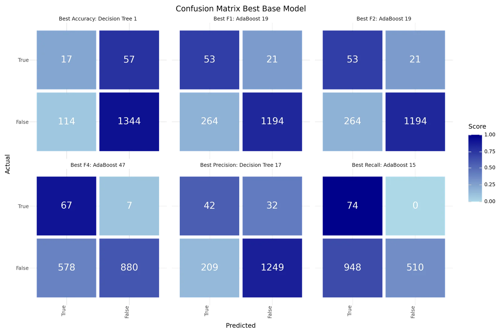
Best base classification models Confusion matrix
5. K Means, DBSCAN and Agglomerative Clustering
Having understood the complexity of the data we will try to segment the data into clusters, which we plan to use in our improvement approaches for the classification models. We will apply three different clustering algorithms K Means, DBSCAN (Density-Based Spatial Clustering of Applications with Noise) and Agglomerative Clustering. For all methods we will include All Features but not the target variable Stroke. As a result we will enrich our dataset with one column per approach that defines the Cluster of the record. In case of DBSCAN we can also record a negative one as marker for noise not belonging to any cluster. The three clustering approaches are KMeans, DBSCAN and Agglomerative Clustering.
KMeans
We will perform KMeans clustering over all features of the dataset and determine the best K as number of clusters. First we will apply a StandardScaler and recode all categorical features to numeric format.
| count | mean | std | min | 25% | 50% | 75% | max | |
|---|---|---|---|---|---|---|---|---|
| gender | 5104.0 | 0.0 | 1.0 | -0.840 | -0.840 | -0.840 | 1.188 | 3.217 |
| age | 5104.0 | -0.0 | 1.0 | -1.910 | -0.807 | 0.077 | 0.785 | 1.714 |
| hypertension | 5104.0 | -0.0 | 1.0 | -0.328 | -0.328 | -0.328 | -0.328 | 3.051 |
| heart_disease | 5104.0 | 0.0 | 1.0 | -0.239 | -0.239 | -0.239 | -0.239 | 4.182 |
| ever_married | 5104.0 | -0.0 | 1.0 | -1.383 | -1.383 | 0.723 | 0.723 | 0.723 |
| work_type | 5104.0 | -0.0 | 1.0 | -1.988 | -0.153 | -0.153 | 0.764 | 1.681 |
| Residence_type | 5104.0 | 0.0 | 1.0 | -1.017 | -1.017 | 0.984 | 0.984 | 0.984 |
| smoking_status | 5104.0 | -0.0 | 1.0 | -1.286 | -1.286 | 0.581 | 0.581 | 1.515 |
| glucose_group | 5104.0 | 0.0 | 1.0 | -0.412 | -0.412 | -0.412 | -0.412 | 2.945 |
| bmi_group | 5104.0 | -0.0 | 1.0 | -2.129 | -1.079 | -0.030 | 1.020 | 1.020 |
Below you can see the resulting graph showing inertia values over number of clusters K.
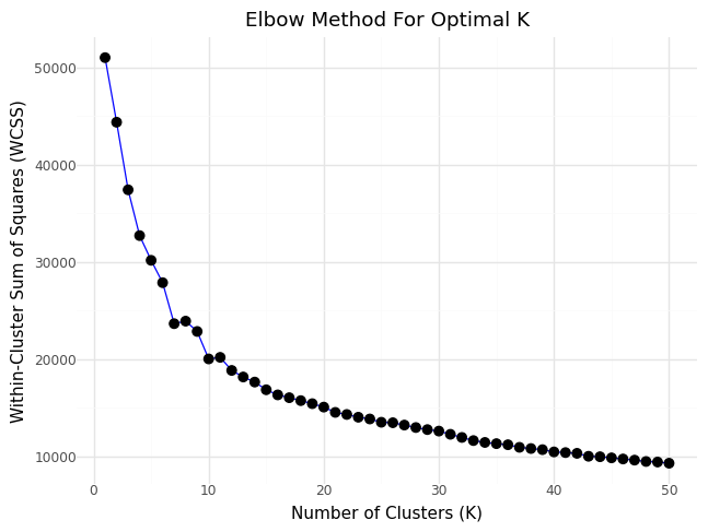
Elbow curve - Inertia over number of clusters
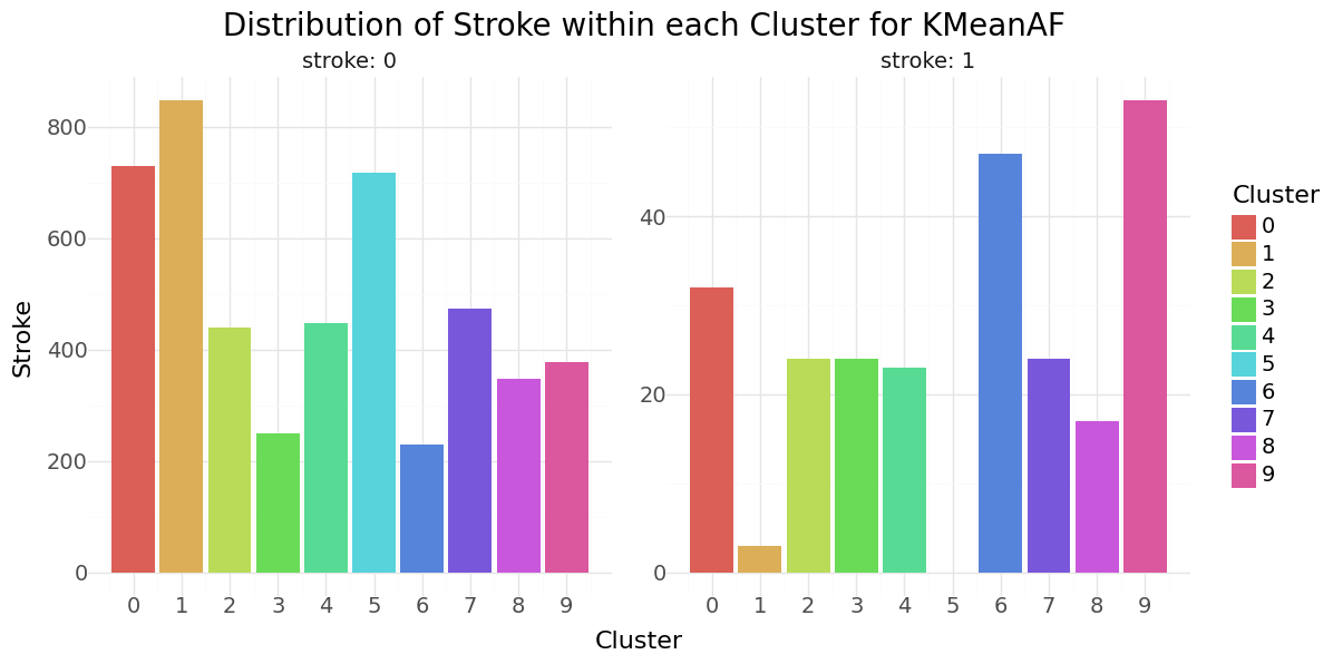
From the ellbow curve we identify K=10 as significant candidate for the ellbow point and will rerun KMean for K=9 and include it in our data set. Below you can see the resulting distributions for the continuos variable Age as Violinplot differentiated by cluster, as well as the Distribution for the categorical variables for Heart Disease, Hypertension.
| KMeanAF | Total | Stroke | Not_Stroke | |
|---|---|---|---|---|
| 0 | 0 | 761 | 32 | 729 |
| 1 | 1 | 850 | 3 | 847 |
| 2 | 2 | 463 | 24 | 439 |
| 3 | 3 | 274 | 24 | 250 |
| 4 | 4 | 470 | 23 | 447 |
| 5 | 5 | 717 | 0 | 717 |
| 6 | 6 | 276 | 47 | 229 |
| 7 | 7 | 498 | 24 | 474 |
| 8 | 8 | 364 | 17 | 347 |
| 9 | 9 | 431 | 53 | 378 |
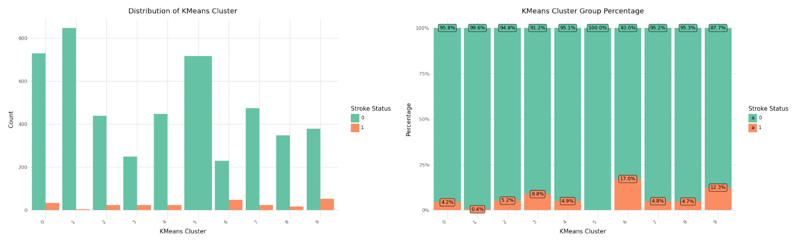
Cluster distribution
We can see that cluster label 5 has patients segmented without stroke. Cluster label 6 shows the highest percentage of stroke cases per segment. Below you can see the resulting distributions for the continuos variables Age, Avg Glucose Level and BMI as Violinplot differentiated by cluster, as well as the Distribution for the categorical variables for Heart Disease, Hypertension.
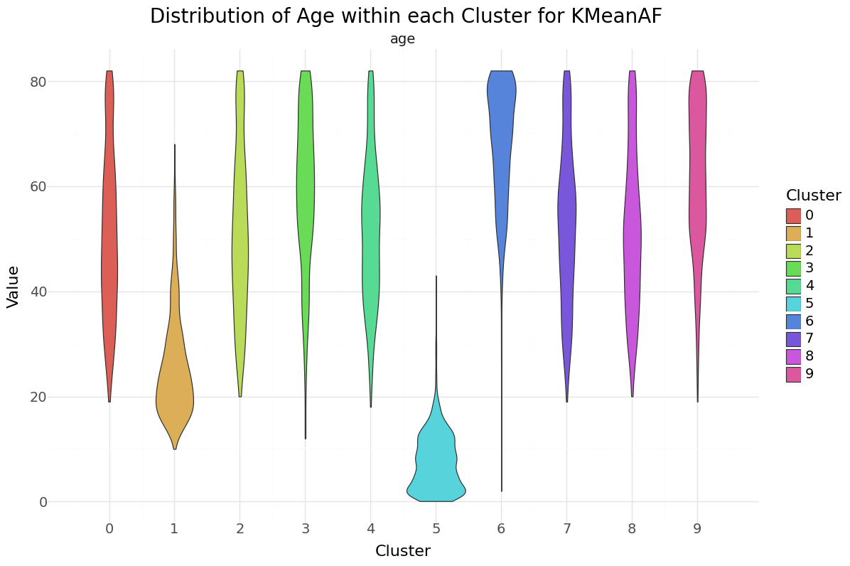
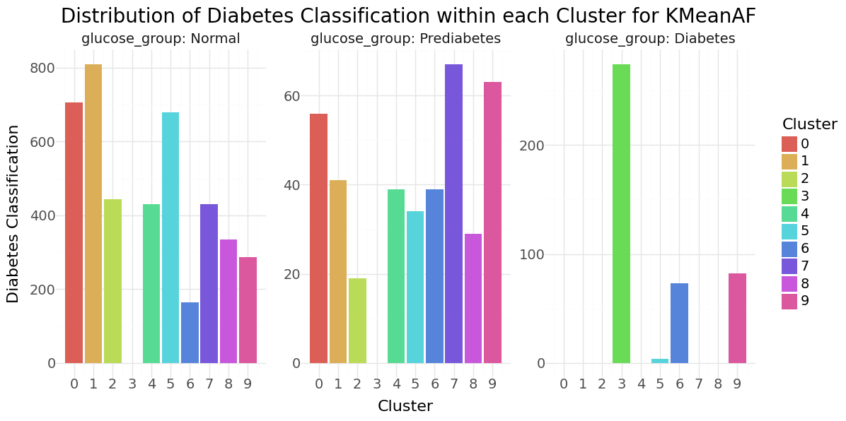
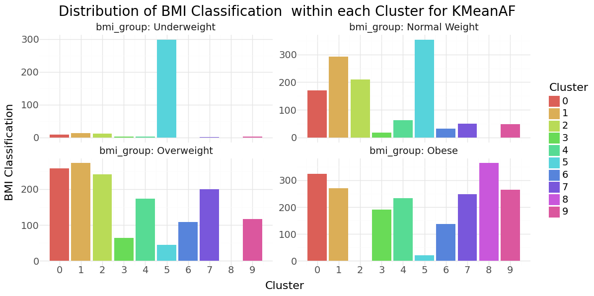
KMean cluster - Distribution of Age, Glucose and BMI Groups
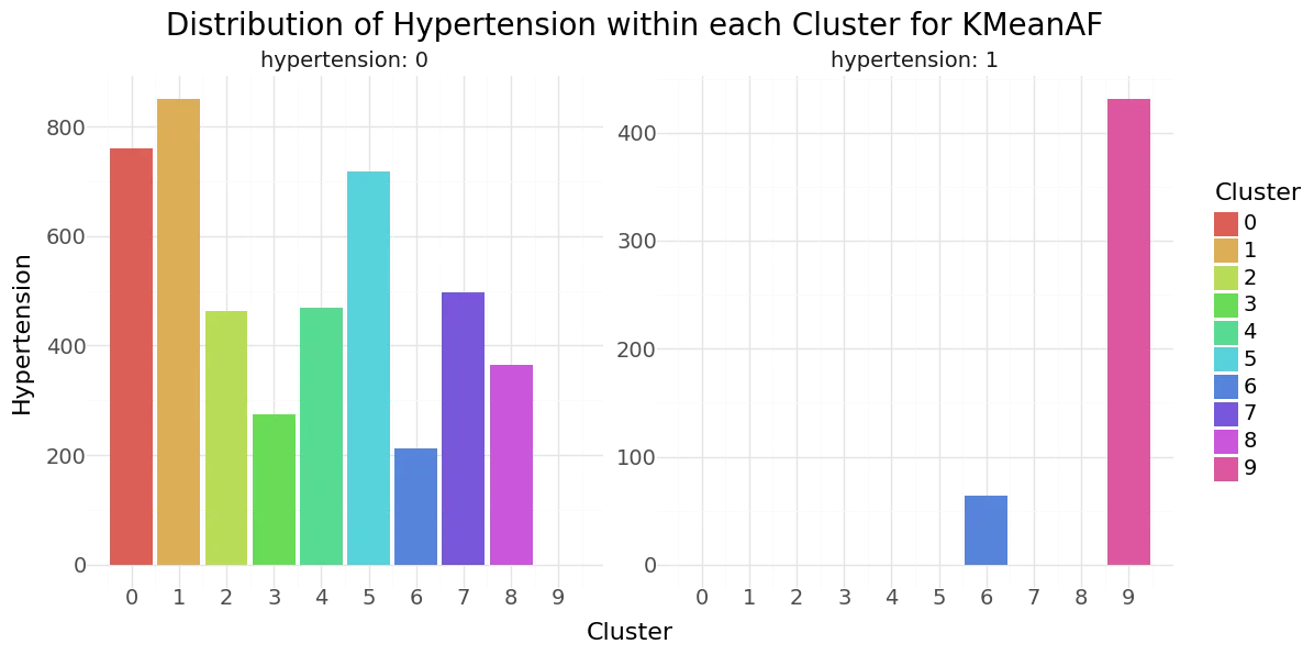
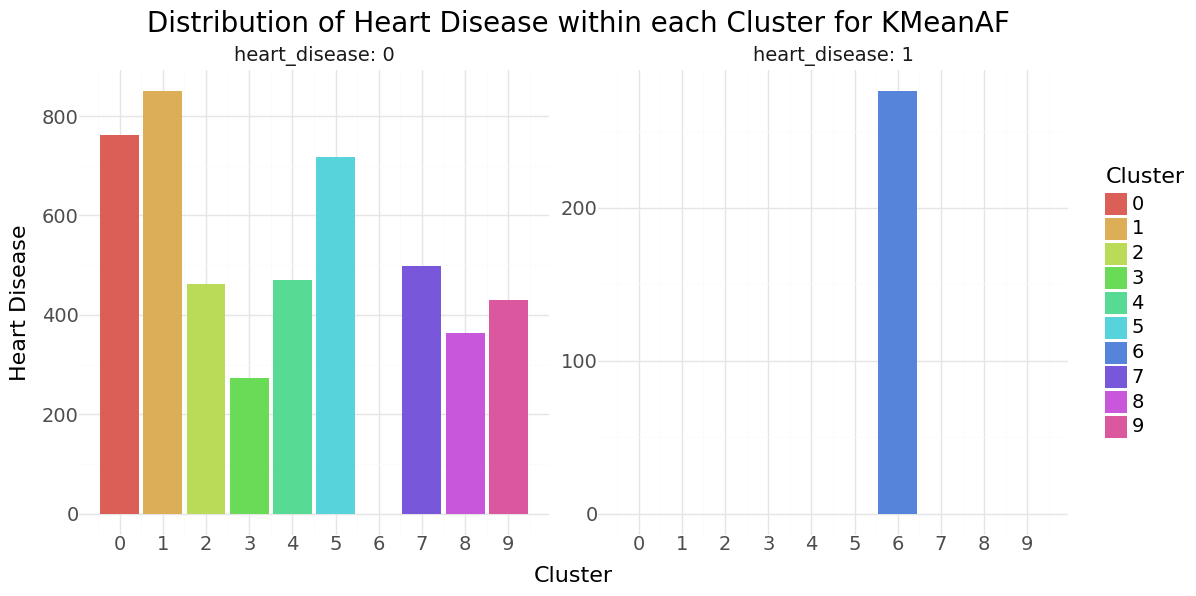
KMean cluster - Distribution of Hypertension, Heart disease and Stroke
DBSCAN
Next we will perform DBSCAN clustering over all features of the dataset and determine. The number of clusters are optimized by DBSCAN itself. As before, we will apply a StandardScaler and recode all categorical features to numeric format.
| count | mean | std | min | 25% | 50% | 75% | max | |
|---|---|---|---|---|---|---|---|---|
| gender | 5104.0 | 0.0 | 1.0 | -0.840 | -0.840 | -0.840 | 1.188 | 3.217 |
| age | 5104.0 | -0.0 | 1.0 | -1.910 | -0.807 | 0.077 | 0.785 | 1.714 |
| hypertension | 5104.0 | -0.0 | 1.0 | -0.328 | -0.328 | -0.328 | -0.328 | 3.051 |
| heart_disease | 5104.0 | 0.0 | 1.0 | -0.239 | -0.239 | -0.239 | -0.239 | 4.182 |
| ever_married | 5104.0 | -0.0 | 1.0 | -1.383 | -1.383 | 0.723 | 0.723 | 0.723 |
| work_type | 5104.0 | -0.0 | 1.0 | -1.988 | -0.153 | -0.153 | 0.764 | 1.681 |
| Residence_type | 5104.0 | 0.0 | 1.0 | -1.017 | -1.017 | 0.984 | 0.984 | 0.984 |
| smoking_status | 5104.0 | -0.0 | 1.0 | -1.286 | -1.286 | 0.581 | 0.581 | 1.515 |
| glucose_group | 5104.0 | 0.0 | 1.0 | -0.412 | -0.412 | -0.412 | -0.412 | 2.945 |
| bmi_group | 5104.0 | -0.0 | 1.0 | -2.129 | -1.079 | -0.030 | 1.020 | 1.020 |
Below you can see the result. DBSCAN calculated 4 clusters and identified 2 records as noise.
| DBSCANAF | Total | Stroke | Not_Stroke | |
|---|---|---|---|---|
| 0 | -1 | 3 | 0 | 3 |
| 1 | 0 | 211 | 34 | 177 |
| 2 | 1 | 4397 | 147 | 4250 |
| 3 | 2 | 431 | 53 | 378 |
| 4 | 3 | 62 | 13 | 49 |
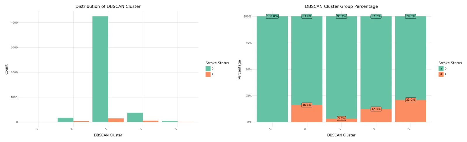
Cluster distribution
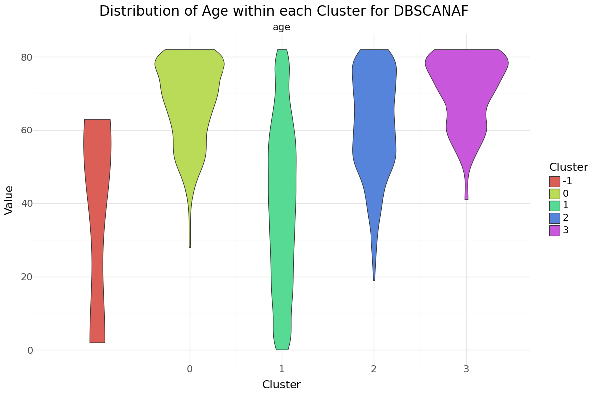
We can see that cluster label 1 has the majority of all observations and also the smallest stroke percentage.There were three observations classified as noise, all non stroke patients. Below you can see the resulting distributions for the continuos variables Age, Avg Glucose Level and BMI as Violinplot differentiated by cluster, as well as the Distribution for the categorical variables for Heart Disease, Hypertension.
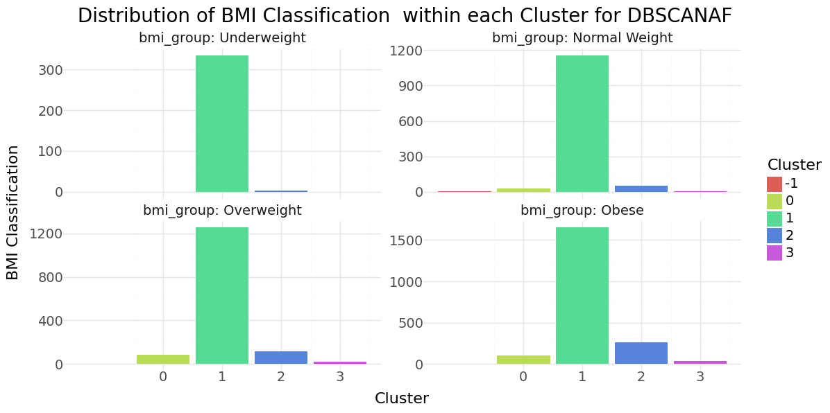
DBSCAN cluster-distribution for Age, glucose level and bmi
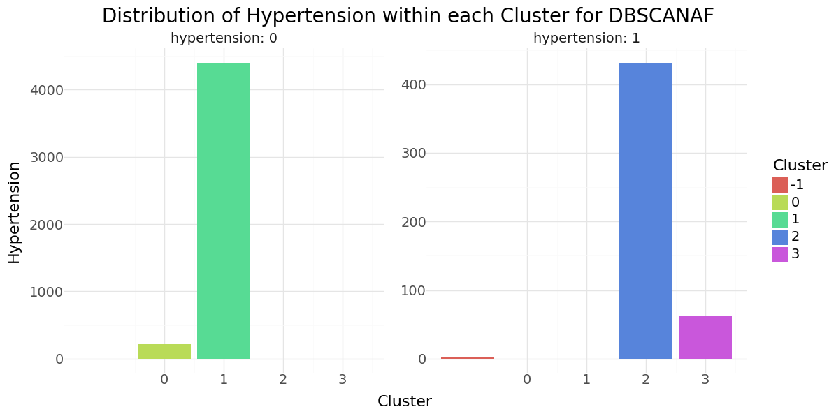
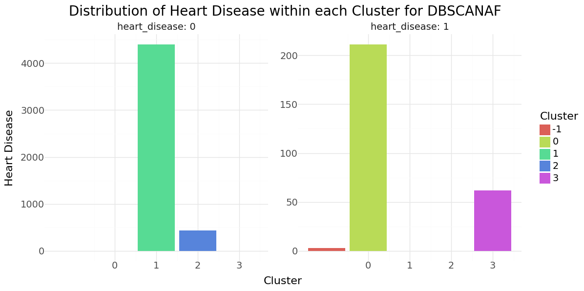
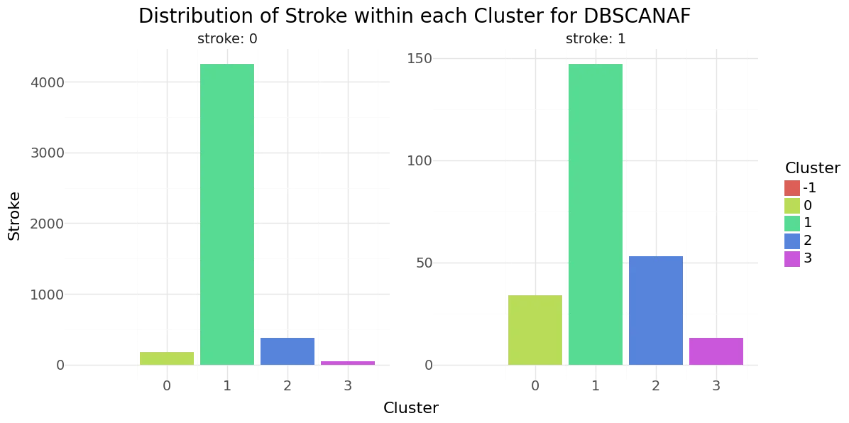
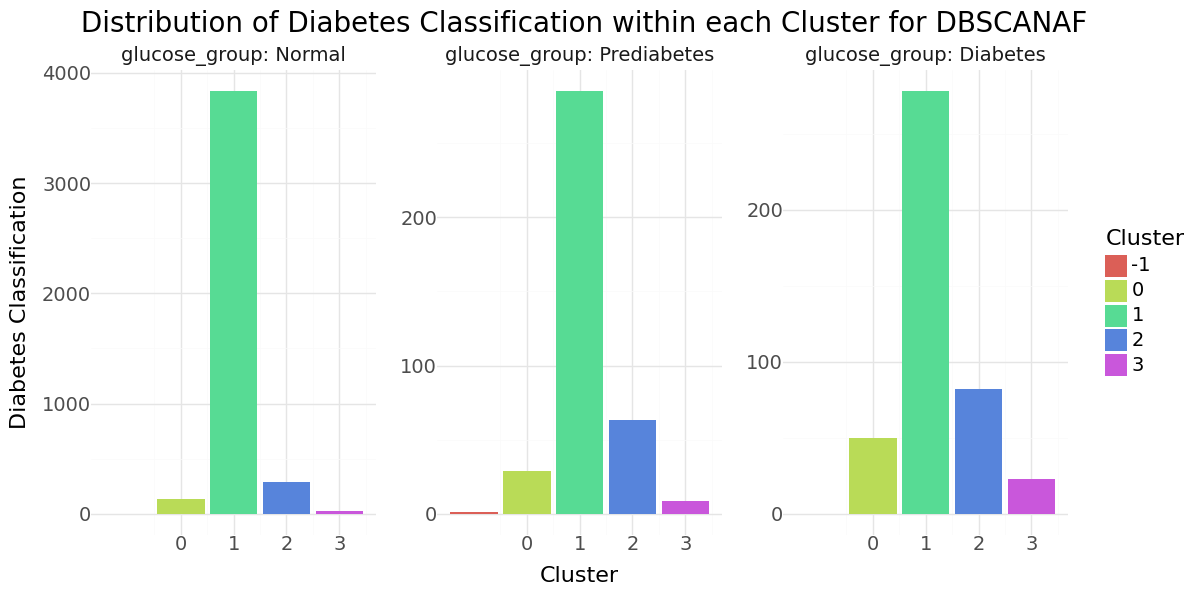
DBSCAN cluster-distribution for Hypertension, Heart disease and stroke
Agglomerative Clustering SF
Next we will perform Agglomerative Clustering over all features of the dataset and determine the best n as number of clusters. As before, we will apply a StandardScaler and recode all categorical features to numeric format.
| count | mean | std | min | 25% | 50% | 75% | max | |
|---|---|---|---|---|---|---|---|---|
| gender | 5104.0 | 0.0 | 1.0 | -0.840 | -0.840 | -0.840 | 1.188 | 3.217 |
| age | 5104.0 | -0.0 | 1.0 | -1.910 | -0.807 | 0.077 | 0.785 | 1.714 |
| hypertension | 5104.0 | -0.0 | 1.0 | -0.328 | -0.328 | -0.328 | -0.328 | 3.051 |
| heart_disease | 5104.0 | 0.0 | 1.0 | -0.239 | -0.239 | -0.239 | -0.239 | 4.182 |
| ever_married | 5104.0 | -0.0 | 1.0 | -1.383 | -1.383 | 0.723 | 0.723 | 0.723 |
| work_type | 5104.0 | -0.0 | 1.0 | -1.988 | -0.153 | -0.153 | 0.764 | 1.681 |
| Residence_type | 5104.0 | 0.0 | 1.0 | -1.017 | -1.017 | 0.984 | 0.984 | 0.984 |
| smoking_status | 5104.0 | -0.0 | 1.0 | -1.286 | -1.286 | 0.581 | 0.581 | 1.515 |
| glucose_group | 5104.0 | 0.0 | 1.0 | -0.412 | -0.412 | -0.412 | -0.412 | 2.945 |
| bmi_group | 5104.0 | -0.0 | 1.0 | -2.129 | -1.079 | -0.030 | 1.020 | 1.020 |
Below you can see the resulting graph showing silhouettes scores over number of clusters n for the selected features.
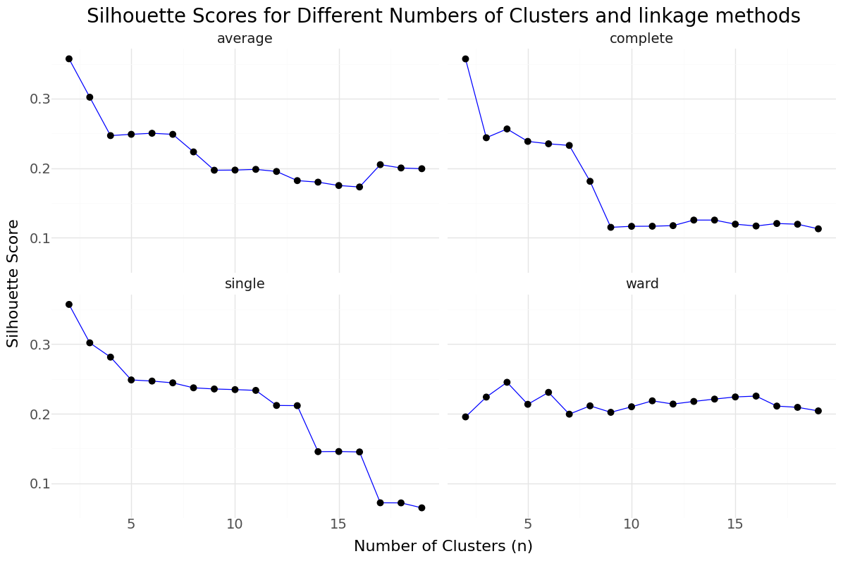
Silhouettes Scores for different linkage parameters
For the selected features we select n=9 as best candidate and will rerun the Agglomerative Clustering for n=9 and ward linkage and include it in our data set. Below you can see the resulting distribution and cluster counts.
| AggloAF | Total | Stroke | Not_Stroke | |
|---|---|---|---|---|
| 0 | 0 | 966 | 13 | 953 |
| 1 | 1 | 645 | 0 | 645 |
| 2 | 2 | 696 | 35 | 661 |
| 3 | 3 | 431 | 53 | 378 |
| 4 | 4 | 587 | 21 | 566 |
| 5 | 5 | 505 | 42 | 463 |
| 6 | 6 | 276 | 47 | 229 |
| 7 | 7 | 377 | 11 | 366 |
| 8 | 8 | 621 | 25 | 596 |
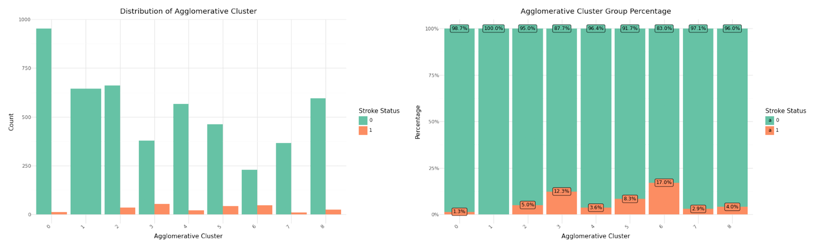
Cluster distribution
We can see that cluster label 1 has patients segmented without stroke. Cluster label 6 shows the highest percentage of stroke cases per segment. Below you can see the resulting distributions for the continuos variables Age, Avg Glucose Level and BMI as Violinplot differentiated by cluster, as well as the Distribution for the categorical variables for Heart Disease, Hypertension.
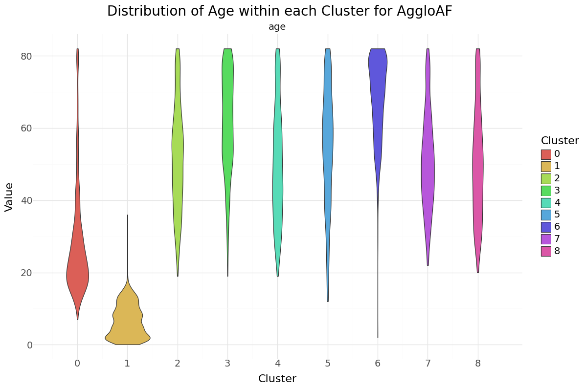
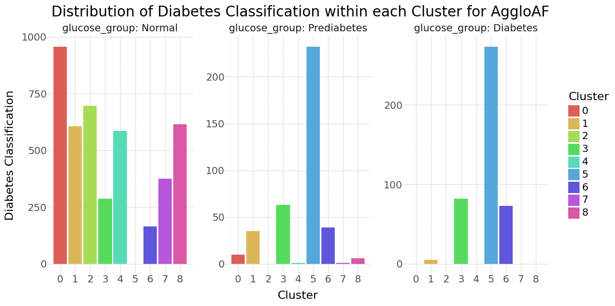
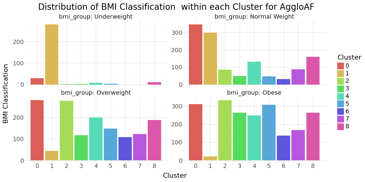
Agglomerative Clustering cluster-distribution for Age, glucose level and bmi
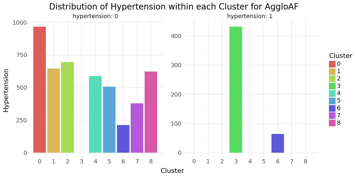
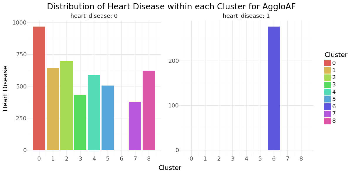
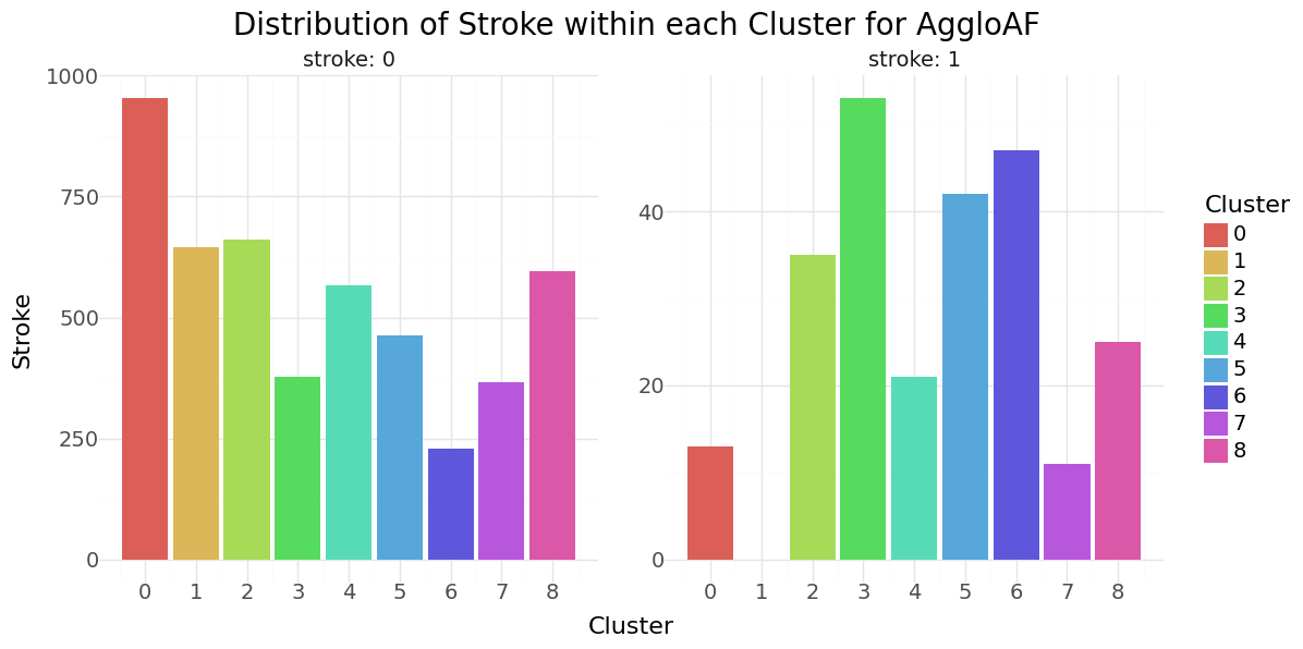
Agglomerative Clustering cluster-distribution for Hypertension, Heart disease and stroke
Cluster based classification
We can now analyze the quality of the clusters and use the results to create additional features and use these clusters as part of the feature set for classification. We will apply the same classification algorithms as for the base models and will apply resampling methods as before. The table below shows the results for models with a recall of greater than 0.7.
| Clustering | Resampling | Scoring | Model | Precision | Recall | Accuracy | F1 | F2 | F4 | |
|---|---|---|---|---|---|---|---|---|---|---|
| 83 | AggloAF | TomekLinks | f1 | AdaBoost | 0.167 | 0.703 | 0.816 | 0.269 | 0.428 | 0.591 |
| 51 | DBSCANAF | TomekLinks | f1 | AdaBoost | 0.154 | 0.703 | 0.799 | 0.253 | 0.411 | 0.581 |
| 59 | DBSCANAF | TomekLinks | f2 | AdaBoost | 0.133 | 0.743 | 0.752 | 0.225 | 0.387 | 0.585 |
| 60 | DBSCANAF | TomekLinks | f4 | Logistic Regression | 0.130 | 0.716 | 0.754 | 0.220 | 0.376 | 0.566 |
| 56 | DBSCANAF | TomekLinks | f2 | Logistic Regression | 0.130 | 0.716 | 0.754 | 0.220 | 0.376 | 0.566 |
| 95 | AggloAF | TomekLinks | f4 | AdaBoost | 0.118 | 0.824 | 0.694 | 0.206 | 0.375 | 0.610 |
| 91 | AggloAF | TomekLinks | f2 | AdaBoost | 0.118 | 0.824 | 0.694 | 0.206 | 0.375 | 0.610 |
| 27 | KMeanAF | TomekLinks | f2 | AdaBoost | 0.116 | 0.824 | 0.687 | 0.203 | 0.371 | 0.606 |
| 19 | KMeanAF | TomekLinks | f1 | AdaBoost | 0.116 | 0.824 | 0.687 | 0.203 | 0.371 | 0.606 |
| 31 | KMeanAF | TomekLinks | f4 | AdaBoost | 0.116 | 0.824 | 0.687 | 0.203 | 0.371 | 0.606 |
| 48 | DBSCANAF | TomekLinks | f1 | Logistic Regression | 0.121 | 0.757 | 0.722 | 0.208 | 0.368 | 0.578 |
| 20 | KMeanAF | TomekLinks | recall | Logistic Regression | 0.109 | 0.892 | 0.644 | 0.195 | 0.367 | 0.628 |
| 28 | KMeanAF | TomekLinks | f4 | Logistic Regression | 0.109 | 0.892 | 0.644 | 0.195 | 0.367 | 0.628 |
| 24 | KMeanAF | TomekLinks | f2 | Logistic Regression | 0.109 | 0.892 | 0.644 | 0.195 | 0.367 | 0.628 |
| 16 | KMeanAF | TomekLinks | f1 | Logistic Regression | 0.109 | 0.892 | 0.644 | 0.195 | 0.367 | 0.628 |
| 63 | DBSCANAF | TomekLinks | f4 | AdaBoost | 0.106 | 0.919 | 0.620 | 0.189 | 0.362 | 0.632 |
| 21 | KMeanAF | TomekLinks | recall | Decision Tree | 0.113 | 0.784 | 0.692 | 0.197 | 0.358 | 0.581 |
| 66 | AggloAF | Adasyn | f1 | Naive Bayes | 0.112 | 0.784 | 0.689 | 0.196 | 0.356 | 0.579 |
| 89 | AggloAF | TomekLinks | f2 | Decision Tree | 0.117 | 0.716 | 0.726 | 0.202 | 0.354 | 0.551 |
| 75 | AggloAF | Adasyn | f2 | AdaBoost | 0.102 | 0.919 | 0.605 | 0.184 | 0.353 | 0.625 |
| 26 | KMeanAF | TomekLinks | f2 | Naive Bayes | 0.106 | 0.770 | 0.676 | 0.187 | 0.342 | 0.563 |
| 18 | KMeanAF | TomekLinks | f1 | Naive Bayes | 0.106 | 0.770 | 0.676 | 0.187 | 0.342 | 0.563 |
| 15 | KMeanAF | Adasyn | f4 | AdaBoost | 0.093 | 0.932 | 0.560 | 0.170 | 0.334 | 0.610 |
| 11 | KMeanAF | Adasyn | f2 | AdaBoost | 0.093 | 0.932 | 0.560 | 0.170 | 0.334 | 0.610 |
| 43 | DBSCANAF | Adasyn | f2 | AdaBoost | 0.095 | 0.892 | 0.584 | 0.172 | 0.333 | 0.597 |
| 94 | AggloAF | TomekLinks | f4 | Naive Bayes | 0.094 | 0.905 | 0.573 | 0.170 | 0.332 | 0.600 |
| 80 | AggloAF | TomekLinks | f1 | Logistic Regression | 0.091 | 0.932 | 0.547 | 0.166 | 0.327 | 0.604 |
| 62 | DBSCANAF | TomekLinks | f4 | Naive Bayes | 0.093 | 0.838 | 0.596 | 0.167 | 0.322 | 0.569 |
| 30 | KMeanAF | TomekLinks | f4 | Naive Bayes | 0.084 | 0.946 | 0.496 | 0.154 | 0.309 | 0.589 |
| 79 | AggloAF | Adasyn | f4 | AdaBoost | 0.079 | 0.986 | 0.445 | 0.146 | 0.299 | 0.589 |
| 34 | DBSCANAF | Adasyn | f1 | Naive Bayes | 0.085 | 0.784 | 0.580 | 0.153 | 0.296 | 0.528 |
| 47 | DBSCANAF | Adasyn | f4 | AdaBoost | 0.074 | 1.000 | 0.398 | 0.138 | 0.287 | 0.577 |
| 14 | KMeanAF | Adasyn | f4 | Naive Bayes | 0.075 | 0.959 | 0.428 | 0.139 | 0.286 | 0.567 |
| 6 | KMeanAF | Adasyn | recall | Naive Bayes | 0.075 | 0.959 | 0.428 | 0.139 | 0.286 | 0.567 |
| 42 | DBSCANAF | Adasyn | f2 | Naive Bayes | 0.076 | 0.865 | 0.483 | 0.139 | 0.280 | 0.536 |
| 10 | KMeanAF | Adasyn | f2 | Naive Bayes | 0.078 | 0.811 | 0.525 | 0.142 | 0.280 | 0.521 |
| 22 | KMeanAF | TomekLinks | recall | Naive Bayes | 0.070 | 1.000 | 0.362 | 0.131 | 0.274 | 0.563 |
| 46 | DBSCANAF | Adasyn | f4 | Naive Bayes | 0.070 | 0.932 | 0.401 | 0.131 | 0.270 | 0.542 |
| 7 | KMeanAF | Adasyn | recall | AdaBoost | 0.068 | 1.000 | 0.336 | 0.127 | 0.267 | 0.553 |
| 78 | AggloAF | Adasyn | f4 | Naive Bayes | 0.064 | 0.973 | 0.315 | 0.121 | 0.254 | 0.531 |
| 74 | AggloAF | Adasyn | f2 | Naive Bayes | 0.065 | 0.905 | 0.366 | 0.121 | 0.252 | 0.514 |
| 70 | AggloAF | Adasyn | recall | Naive Bayes | 0.061 | 0.973 | 0.279 | 0.115 | 0.245 | 0.519 |
| 55 | DBSCANAF | TomekLinks | recall | AdaBoost | 0.059 | 1.000 | 0.233 | 0.112 | 0.239 | 0.517 |
| Clustering | Resampling | Scoring | Model | F4 | True 1 | True 0 | False 1 | False 0 | |
|---|---|---|---|---|---|---|---|---|---|
| 83 | AggloAF | TomekLinks | f1 | AdaBoost | 0.591 | 52 | 1198 | 260 | 22 |
| 51 | DBSCANAF | TomekLinks | f1 | AdaBoost | 0.581 | 52 | 1172 | 285 | 22 |
| 59 | DBSCANAF | TomekLinks | f2 | AdaBoost | 0.585 | 55 | 1097 | 360 | 19 |
| 60 | DBSCANAF | TomekLinks | f4 | Logistic Regression | 0.566 | 53 | 1102 | 355 | 21 |
| 56 | DBSCANAF | TomekLinks | f2 | Logistic Regression | 0.566 | 53 | 1102 | 355 | 21 |
| 95 | AggloAF | TomekLinks | f4 | AdaBoost | 0.610 | 61 | 1002 | 456 | 13 |
| 91 | AggloAF | TomekLinks | f2 | AdaBoost | 0.610 | 61 | 1002 | 456 | 13 |
| 27 | KMeanAF | TomekLinks | f2 | AdaBoost | 0.606 | 61 | 992 | 466 | 13 |
| 19 | KMeanAF | TomekLinks | f1 | AdaBoost | 0.606 | 61 | 992 | 466 | 13 |
| 31 | KMeanAF | TomekLinks | f4 | AdaBoost | 0.606 | 61 | 992 | 466 | 13 |
| 48 | DBSCANAF | TomekLinks | f1 | Logistic Regression | 0.578 | 56 | 1049 | 408 | 18 |
| 20 | KMeanAF | TomekLinks | recall | Logistic Regression | 0.628 | 66 | 921 | 537 | 8 |
| 28 | KMeanAF | TomekLinks | f4 | Logistic Regression | 0.628 | 66 | 921 | 537 | 8 |
| 24 | KMeanAF | TomekLinks | f2 | Logistic Regression | 0.628 | 66 | 921 | 537 | 8 |
| 16 | KMeanAF | TomekLinks | f1 | Logistic Regression | 0.628 | 66 | 921 | 537 | 8 |
| 63 | DBSCANAF | TomekLinks | f4 | AdaBoost | 0.632 | 68 | 881 | 576 | 6 |
| 21 | KMeanAF | TomekLinks | recall | Decision Tree | 0.581 | 58 | 1002 | 456 | 16 |
| 66 | AggloAF | Adasyn | f1 | Naive Bayes | 0.579 | 58 | 997 | 461 | 16 |
| 89 | AggloAF | TomekLinks | f2 | Decision Tree | 0.551 | 53 | 1059 | 399 | 21 |
| 75 | AggloAF | Adasyn | f2 | AdaBoost | 0.625 | 68 | 859 | 599 | 6 |
| 26 | KMeanAF | TomekLinks | f2 | Naive Bayes | 0.563 | 57 | 978 | 480 | 17 |
| 18 | KMeanAF | TomekLinks | f1 | Naive Bayes | 0.563 | 57 | 978 | 480 | 17 |
| 15 | KMeanAF | Adasyn | f4 | AdaBoost | 0.610 | 69 | 789 | 669 | 5 |
| 11 | KMeanAF | Adasyn | f2 | AdaBoost | 0.610 | 69 | 789 | 669 | 5 |
| 43 | DBSCANAF | Adasyn | f2 | AdaBoost | 0.597 | 66 | 828 | 629 | 8 |
| 94 | AggloAF | TomekLinks | f4 | Naive Bayes | 0.600 | 67 | 811 | 647 | 7 |
| 80 | AggloAF | TomekLinks | f1 | Logistic Regression | 0.604 | 69 | 769 | 689 | 5 |
| 62 | DBSCANAF | TomekLinks | f4 | Naive Bayes | 0.569 | 62 | 851 | 606 | 12 |
| 30 | KMeanAF | TomekLinks | f4 | Naive Bayes | 0.589 | 70 | 690 | 768 | 4 |
| 79 | AggloAF | Adasyn | f4 | AdaBoost | 0.589 | 73 | 608 | 850 | 1 |
| 34 | DBSCANAF | Adasyn | f1 | Naive Bayes | 0.528 | 58 | 830 | 627 | 16 |
| 47 | DBSCANAF | Adasyn | f4 | AdaBoost | 0.577 | 74 | 536 | 921 | 0 |
| 14 | KMeanAF | Adasyn | f4 | Naive Bayes | 0.567 | 71 | 585 | 873 | 3 |
| 6 | KMeanAF | Adasyn | recall | Naive Bayes | 0.567 | 71 | 585 | 873 | 3 |
| 42 | DBSCANAF | Adasyn | f2 | Naive Bayes | 0.536 | 64 | 676 | 781 | 10 |
| 10 | KMeanAF | Adasyn | f2 | Naive Bayes | 0.521 | 60 | 744 | 714 | 14 |
| 22 | KMeanAF | TomekLinks | recall | Naive Bayes | 0.563 | 74 | 480 | 978 | 0 |
| 46 | DBSCANAF | Adasyn | f4 | Naive Bayes | 0.542 | 69 | 545 | 912 | 5 |
| 7 | KMeanAF | Adasyn | recall | AdaBoost | 0.553 | 74 | 440 | 1018 | 0 |
| 78 | AggloAF | Adasyn | f4 | Naive Bayes | 0.531 | 72 | 410 | 1048 | 2 |
| 74 | AggloAF | Adasyn | f2 | Naive Bayes | 0.514 | 67 | 493 | 965 | 7 |
| 70 | AggloAF | Adasyn | recall | Naive Bayes | 0.519 | 72 | 355 | 1103 | 2 |
| 55 | DBSCANAF | TomekLinks | recall | AdaBoost | 0.517 | 74 | 282 | 1175 | 0 |
The best models depending on the scoring metric are shown below.
| Best Accuracy | Best Precision | Best Recall | Best F1 | Best F2 | Best F4 | |
|---|---|---|---|---|---|---|
| Model ID | 84 | 64 | 47 | 83 | 83 | 63 |
| Clustering | AggloAF | AggloAF | DBSCANAF | AggloAF | AggloAF | DBSCANAF |
| Resampling | TomekLinks | Adasyn | Adasyn | TomekLinks | TomekLinks | TomekLinks |
| Scoring | recall | f1 | f4 | f1 | f1 | f4 |
| Model | Logistic Reg | Logistic Reg | AdaBoost | AdaBoost | AdaBoost | AdaBoost |
| Precision | 0.0 | 0.1901 | 0.0744 | 0.1667 | 0.1667 | 0.1056 |
| Recall | 0.0 | 0.3108 | 1.0 | 0.7027 | 0.7027 | 0.9189 |
| Accuracy | 0.9517 | 0.9027 | 0.3984 | 0.8159 | 0.8159 | 0.6199 |
| F1 | 0.0 | 0.2359 | 0.1384 | 0.2694 | 0.2694 | 0.1894 |
| F2 | 0.0 | 0.2758 | 0.2866 | 0.4276 | 0.4276 | 0.3617 |
| F4 | 0.0 | 0.2996 | 0.5773 | 0.5909 | 0.5909 | 0.6324 |
| True 1 | 0 | 23 | 74 | 52 | 52 | 68 |
| True 0 | 1458 | 1360 | 536 | 1198 | 1198 | 881 |
| False 1 | 0 | 98 | 921 | 260 | 260 | 576 |
| False 0 | 74 | 51 | 0 | 22 | 22 | 6 |

Confusion matrix - Best models for Cluster based Classification
Cluster only classification
Next we will evaluate the clustering results using only the cluster labels as feature and the stroke variable as target.
| Clustering | Resampling | Scoring | Model | Precision | Recall | Accuracy | F1 | F2 | F4 | |
|---|---|---|---|---|---|---|---|---|---|---|
| 1 | KMeanAF | Adasyn | f1 | Decision Tree | 0.082 | 0.716 | 0.597 | 0.146 | 0.280 | 0.491 |
| 9 | KMeanAF | Adasyn | f2 | Decision Tree | 0.082 | 0.716 | 0.597 | 0.146 | 0.280 | 0.491 |
| 13 | KMeanAF | Adasyn | f4 | Decision Tree | 0.082 | 0.716 | 0.597 | 0.146 | 0.280 | 0.491 |
| 95 | AggloAF | TomekLinks | f4 | AdaBoost | 0.074 | 0.919 | 0.441 | 0.137 | 0.280 | 0.550 |
| 5 | KMeanAF | Adasyn | recall | Decision Tree | 0.082 | 0.716 | 0.597 | 0.146 | 0.280 | 0.491 |
| 11 | KMeanAF | Adasyn | f2 | AdaBoost | 0.070 | 1.000 | 0.361 | 0.131 | 0.274 | 0.562 |
| 8 | KMeanAF | Adasyn | f2 | Logistic Regression | 0.070 | 1.000 | 0.361 | 0.131 | 0.274 | 0.562 |
| 6 | KMeanAF | Adasyn | recall | Naive Bayes | 0.070 | 1.000 | 0.361 | 0.131 | 0.274 | 0.562 |
| 3 | KMeanAF | Adasyn | f1 | AdaBoost | 0.070 | 1.000 | 0.361 | 0.131 | 0.274 | 0.562 |
| 2 | KMeanAF | Adasyn | f1 | Naive Bayes | 0.070 | 1.000 | 0.361 | 0.131 | 0.274 | 0.562 |
| 10 | KMeanAF | Adasyn | f2 | Naive Bayes | 0.070 | 1.000 | 0.361 | 0.131 | 0.274 | 0.562 |
| 4 | KMeanAF | Adasyn | recall | Logistic Regression | 0.070 | 1.000 | 0.361 | 0.131 | 0.274 | 0.562 |
| 23 | KMeanAF | TomekLinks | recall | AdaBoost | 0.070 | 1.000 | 0.361 | 0.131 | 0.274 | 0.562 |
| 0 | KMeanAF | Adasyn | f1 | Logistic Regression | 0.070 | 1.000 | 0.361 | 0.131 | 0.274 | 0.562 |
| 15 | KMeanAF | Adasyn | f4 | AdaBoost | 0.070 | 1.000 | 0.361 | 0.131 | 0.274 | 0.562 |
| 22 | KMeanAF | TomekLinks | recall | Naive Bayes | 0.070 | 1.000 | 0.361 | 0.131 | 0.274 | 0.562 |
| 30 | KMeanAF | TomekLinks | f4 | Naive Bayes | 0.070 | 1.000 | 0.361 | 0.131 | 0.274 | 0.562 |
| 31 | KMeanAF | TomekLinks | f4 | AdaBoost | 0.070 | 1.000 | 0.361 | 0.131 | 0.274 | 0.562 |
| 12 | KMeanAF | Adasyn | f4 | Logistic Regression | 0.070 | 1.000 | 0.361 | 0.131 | 0.274 | 0.562 |
| 14 | KMeanAF | Adasyn | f4 | Naive Bayes | 0.070 | 1.000 | 0.361 | 0.131 | 0.274 | 0.562 |
| 67 | AggloAF | Adasyn | f1 | AdaBoost | 0.067 | 0.946 | 0.364 | 0.126 | 0.262 | 0.535 |
| 7 | KMeanAF | Adasyn | recall | AdaBoost | 0.057 | 1.000 | 0.198 | 0.108 | 0.232 | 0.506 |
| 84 | AggloAF | TomekLinks | recall | Logistic Regression | 0.056 | 1.000 | 0.187 | 0.106 | 0.229 | 0.502 |
| 94 | AggloAF | TomekLinks | f4 | Naive Bayes | 0.056 | 1.000 | 0.187 | 0.106 | 0.229 | 0.502 |
| 92 | AggloAF | TomekLinks | f4 | Logistic Regression | 0.056 | 1.000 | 0.187 | 0.106 | 0.229 | 0.502 |
| 87 | AggloAF | TomekLinks | recall | AdaBoost | 0.056 | 1.000 | 0.187 | 0.106 | 0.229 | 0.502 |
| 86 | AggloAF | TomekLinks | recall | Naive Bayes | 0.056 | 1.000 | 0.187 | 0.106 | 0.229 | 0.502 |
| 70 | AggloAF | Adasyn | recall | Naive Bayes | 0.056 | 1.000 | 0.187 | 0.106 | 0.229 | 0.502 |
| 79 | AggloAF | Adasyn | f4 | AdaBoost | 0.056 | 1.000 | 0.187 | 0.106 | 0.229 | 0.502 |
| 78 | AggloAF | Adasyn | f4 | Naive Bayes | 0.056 | 1.000 | 0.187 | 0.106 | 0.229 | 0.502 |
| 75 | AggloAF | Adasyn | f2 | AdaBoost | 0.056 | 1.000 | 0.187 | 0.106 | 0.229 | 0.502 |
| 74 | AggloAF | Adasyn | f2 | Naive Bayes | 0.056 | 1.000 | 0.187 | 0.106 | 0.229 | 0.502 |
| 66 | AggloAF | Adasyn | f1 | Naive Bayes | 0.056 | 1.000 | 0.187 | 0.106 | 0.229 | 0.502 |
| 71 | AggloAF | Adasyn | recall | AdaBoost | 0.056 | 1.000 | 0.187 | 0.106 | 0.229 | 0.502 |
| Clustering | Resampling | Scoring | Model | F4 | True 1 | True 0 | False 1 | False 0 | |
|---|---|---|---|---|---|---|---|---|---|
| 1 | KMeanAF | Adasyn | f1 | Decision Tree | 0.491 | 53 | 861 | 597 | 21 |
| 9 | KMeanAF | Adasyn | f2 | Decision Tree | 0.491 | 53 | 861 | 597 | 21 |
| 13 | KMeanAF | Adasyn | f4 | Decision Tree | 0.491 | 53 | 861 | 597 | 21 |
| 95 | AggloAF | TomekLinks | f4 | AdaBoost | 0.550 | 68 | 608 | 850 | 6 |
| 5 | KMeanAF | Adasyn | recall | Decision Tree | 0.491 | 53 | 861 | 597 | 21 |
| 11 | KMeanAF | Adasyn | f2 | AdaBoost | 0.562 | 74 | 479 | 979 | 0 |
| 8 | KMeanAF | Adasyn | f2 | Logistic Regression | 0.562 | 74 | 479 | 979 | 0 |
| 6 | KMeanAF | Adasyn | recall | Naive Bayes | 0.562 | 74 | 479 | 979 | 0 |
| 3 | KMeanAF | Adasyn | f1 | AdaBoost | 0.562 | 74 | 479 | 979 | 0 |
| 2 | KMeanAF | Adasyn | f1 | Naive Bayes | 0.562 | 74 | 479 | 979 | 0 |
| 10 | KMeanAF | Adasyn | f2 | Naive Bayes | 0.562 | 74 | 479 | 979 | 0 |
| 4 | KMeanAF | Adasyn | recall | Logistic Regression | 0.562 | 74 | 479 | 979 | 0 |
| 23 | KMeanAF | TomekLinks | recall | AdaBoost | 0.562 | 74 | 479 | 979 | 0 |
| 0 | KMeanAF | Adasyn | f1 | Logistic Regression | 0.562 | 74 | 479 | 979 | 0 |
| 15 | KMeanAF | Adasyn | f4 | AdaBoost | 0.562 | 74 | 479 | 979 | 0 |
| 22 | KMeanAF | TomekLinks | recall | Naive Bayes | 0.562 | 74 | 479 | 979 | 0 |
| 30 | KMeanAF | TomekLinks | f4 | Naive Bayes | 0.562 | 74 | 479 | 979 | 0 |
| 31 | KMeanAF | TomekLinks | f4 | AdaBoost | 0.562 | 74 | 479 | 979 | 0 |
| 12 | KMeanAF | Adasyn | f4 | Logistic Regression | 0.562 | 74 | 479 | 979 | 0 |
| 14 | KMeanAF | Adasyn | f4 | Naive Bayes | 0.562 | 74 | 479 | 979 | 0 |
| 67 | AggloAF | Adasyn | f1 | AdaBoost | 0.535 | 70 | 488 | 970 | 4 |
| 7 | KMeanAF | Adasyn | recall | AdaBoost | 0.506 | 74 | 230 | 1228 | 0 |
| 84 | AggloAF | TomekLinks | recall | Logistic Regression | 0.502 | 74 | 212 | 1246 | 0 |
| 94 | AggloAF | TomekLinks | f4 | Naive Bayes | 0.502 | 74 | 212 | 1246 | 0 |
| 92 | AggloAF | TomekLinks | f4 | Logistic Regression | 0.502 | 74 | 212 | 1246 | 0 |
| 87 | AggloAF | TomekLinks | recall | AdaBoost | 0.502 | 74 | 212 | 1246 | 0 |
| 86 | AggloAF | TomekLinks | recall | Naive Bayes | 0.502 | 74 | 212 | 1246 | 0 |
| 70 | AggloAF | Adasyn | recall | Naive Bayes | 0.502 | 74 | 212 | 1246 | 0 |
| 79 | AggloAF | Adasyn | f4 | AdaBoost | 0.502 | 74 | 212 | 1246 | 0 |
| 78 | AggloAF | Adasyn | f4 | Naive Bayes | 0.502 | 74 | 212 | 1246 | 0 |
| 75 | AggloAF | Adasyn | f2 | AdaBoost | 0.502 | 74 | 212 | 1246 | 0 |
| 74 | AggloAF | Adasyn | f2 | Naive Bayes | 0.502 | 74 | 212 | 1246 | 0 |
| 66 | AggloAF | Adasyn | f1 | Naive Bayes | 0.502 | 74 | 212 | 1246 | 0 |
| 71 | AggloAF | Adasyn | recall | AdaBoost | 0.502 | 74 | 212 | 1246 | 0 |
The best models depending on the scoring metric are shown below.
| Best Accuracy | Best Precision | Best Recall | Best F1 | Best F2 | Best F4 | |
|---|---|---|---|---|---|---|
| Model ID | 48 | 50 | 0 | 32 | 32 | 0 |
| Clustering | DBSCANAF | DBSCANAF | KMeanAF | DBSCANAF | DBSCANAF | KMeanAF |
| Resampling | TomekLinks | TomekLinks | Adasyn | Adasyn | Adasyn | Adasyn |
| Scoring | f1 | f1 | f1 | f1 | f1 | f1 |
| Model | Logistic Reg | Naive Bayes | Logistic Reg | Logistic Reg | Logistic Reg | Logistic Reg |
| Precision | 0.1636 | 0.188 | 0.0703 | 0.1809 | 0.1809 | 0.0703 |
| Recall | 0.1216 | 0.3378 | 1.0 | 0.4595 | 0.4595 | 1.0 |
| Accuracy | 0.9275 | 0.8975 | 0.361 | 0.8733 | 0.8733 | 0.361 |
| F1 | 0.1395 | 0.2415 | 0.1313 | 0.2595 | 0.2595 | 0.1313 |
| F2 | 0.1282 | 0.2914 | 0.2743 | 0.3512 | 0.3512 | 0.2743 |
| F4 | 0.1235 | 0.3227 | 0.5624 | 0.4213 | 0.4213 | 0.5624 |
| True 1 | 9 | 25 | 74 | 34 | 34 | 74 |
| True 0 | 1411 | 1349 | 479 | 1303 | 1303 | 479 |
| False 1 | 46 | 108 | 979 | 154 | 154 | 979 |
| False 0 | 65 | 49 | 0 | 40 | 40 | 0 |
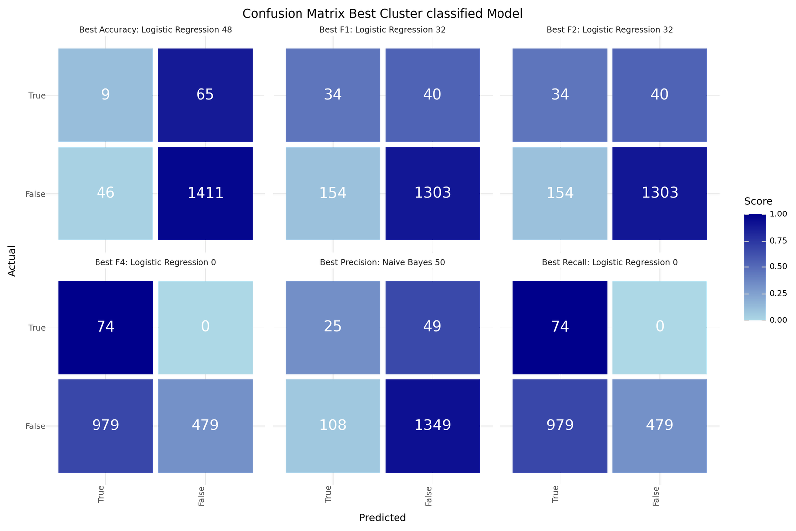
Confusion Matrix - Best models for Cluster only Classification
Classification within the clusters
As suggested we will adjust our approach now and fit classification models for each cluster individually. We evaluated with either over-sampling or no resampling as the size of the clusters would result in small counts of observations with under-sampling. We evaluate the results in two variations:
-
Same model for all clusters: We apply the model sae model to all clusters and calculate the performance based on the aggregated confusion matrix.
-
Best model per cluster: We select the best performing model per cluster label and calculate the performance based on the aggregated confusion matrix.
Results for Same Model for all Cluster
| Clustering | Model | Resampling | Scoring | Precision | Recall | Accuracy | F1 | F2 | F4 | |
|---|---|---|---|---|---|---|---|---|---|---|
| 22 | AggloAF | Logistic Regression | None | f4 | 0.1163 | 0.6667 | 0.7741 | 0.1980 | 0.3425 | 0.5215 |
| 84 | KMeanAF | Logistic Regression | None | f1 | 0.1201 | 0.5811 | 0.8100 | 0.1991 | 0.3287 | 0.4741 |
| 85 | KMeanAF | Logistic Regression | None | f2 | 0.1201 | 0.5811 | 0.8100 | 0.1991 | 0.3287 | 0.4741 |
| 45 | DBSCANAF | Decision Tree | None | f2 | 0.1250 | 0.5541 | 0.7913 | 0.2040 | 0.3285 | 0.4610 |
| 77 | KMeanAF | Decision Tree | None | f2 | 0.1333 | 0.5135 | 0.8446 | 0.2117 | 0.3270 | 0.4398 |
| 44 | DBSCANAF | Decision Tree | None | f1 | 0.1329 | 0.5135 | 0.8147 | 0.2111 | 0.3265 | 0.4395 |
| 86 | KMeanAF | Logistic Regression | None | f4 | 0.1103 | 0.6216 | 0.7809 | 0.1874 | 0.3226 | 0.4884 |
| 29 | AggloAF | Naive Bayes | None | f2 | 0.1242 | 0.5200 | 0.8265 | 0.2005 | 0.3176 | 0.4379 |
| 47 | DBSCANAF | Decision Tree | None | recall | 0.1114 | 0.5541 | 0.7652 | 0.1855 | 0.3087 | 0.4491 |
| 46 | DBSCANAF | Decision Tree | None | f4 | 0.1114 | 0.5541 | 0.7652 | 0.1855 | 0.3087 | 0.4491 |
| 3 | AggloAF | AdaBoost | Adasyn | recall | 0.0996 | 0.6000 | 0.7563 | 0.1708 | 0.2992 | 0.4631 |
| 93 | KMeanAF | Naive Bayes | None | f2 | 0.1176 | 0.4865 | 0.8309 | 0.1895 | 0.2990 | 0.4107 |
| 2 | AggloAF | AdaBoost | Adasyn | f4 | 0.1153 | 0.4933 | 0.8204 | 0.1869 | 0.2979 | 0.4135 |
| 21 | AggloAF | Logistic Regression | None | f2 | 0.0928 | 0.6400 | 0.7234 | 0.1622 | 0.2938 | 0.4752 |
| 23 | AggloAF | Logistic Regression | None | recall | 0.1020 | 0.5467 | 0.7797 | 0.1719 | 0.2920 | 0.4351 |
| 78 | KMeanAF | Decision Tree | None | f4 | 0.1095 | 0.5000 | 0.8144 | 0.1796 | 0.2918 | 0.4133 |
| 61 | DBSCANAF | Naive Bayes | None | f2 | 0.1023 | 0.5405 | 0.7489 | 0.1720 | 0.2911 | 0.4317 |
| 20 | AggloAF | Logistic Regression | None | f1 | 0.0935 | 0.6133 | 0.7351 | 0.1623 | 0.2904 | 0.4622 |
| 94 | KMeanAF | Naive Bayes | None | f4 | 0.1066 | 0.5000 | 0.8094 | 0.1758 | 0.2877 | 0.4108 |
| 33 | DBSCANAF | AdaBoost | Adasyn | f2 | 0.0854 | 0.7027 | 0.6223 | 0.1523 | 0.2873 | 0.4930 |
| 87 | KMeanAF | Logistic Regression | None | recall | 0.1134 | 0.4459 | 0.8358 | 0.1808 | 0.2811 | 0.3803 |
| 79 | KMeanAF | Decision Tree | None | recall | 0.1016 | 0.5000 | 0.8001 | 0.1689 | 0.2803 | 0.4063 |
| 62 | DBSCANAF | Naive Bayes | None | f4 | 0.0817 | 0.6622 | 0.6243 | 0.1454 | 0.2734 | 0.4669 |
| 30 | AggloAF | Naive Bayes | None | f4 | 0.0870 | 0.5600 | 0.7356 | 0.1505 | 0.2682 | 0.4242 |
| 67 | KMeanAF | AdaBoost | Adasyn | recall | 0.1006 | 0.4595 | 0.8111 | 0.1650 | 0.2681 | 0.3798 |
| 95 | KMeanAF | Naive Bayes | None | recall | 0.0823 | 0.6081 | 0.7084 | 0.1449 | 0.2669 | 0.4419 |
| 91 | KMeanAF | Naive Bayes | Adasyn | recall | 0.0751 | 0.5676 | 0.6985 | 0.1327 | 0.2456 | 0.4096 |
| 27 | AggloAF | Naive Bayes | Adasyn | recall | 0.0743 | 0.5733 | 0.6832 | 0.1315 | 0.2446 | 0.4109 |
| 89 | KMeanAF | Naive Bayes | Adasyn | f2 | 0.0752 | 0.5541 | 0.7051 | 0.1325 | 0.2438 | 0.4031 |
| 90 | KMeanAF | Naive Bayes | Adasyn | f4 | 0.0750 | 0.5541 | 0.7040 | 0.1320 | 0.2432 | 0.4027 |
| 38 | DBSCANAF | AdaBoost | None | f4 | 0.0673 | 0.6622 | 0.5408 | 0.1222 | 0.2393 | 0.4357 |
| 39 | DBSCANAF | AdaBoost | None | recall | 0.0673 | 0.6622 | 0.5408 | 0.1222 | 0.2393 | 0.4357 |
| 56 | DBSCANAF | Naive Bayes | Adasyn | f1 | 0.0643 | 0.6216 | 0.5453 | 0.1166 | 0.2275 | 0.4118 |
| 70 | KMeanAF | AdaBoost | None | f4 | 0.0662 | 0.5270 | 0.6787 | 0.1176 | 0.2203 | 0.3739 |
| Clustering | Model | Resampling | Scoring | F2 | True 1 | True 0 | False 1 | False 0 | |
|---|---|---|---|---|---|---|---|---|---|
| 22 | AggloAF | Logistic Regression | None | f4 | 0.3425 | 50 | 1338 | 380 | 25 |
| 84 | KMeanAF | Logistic Regression | None | f1 | 0.3287 | 43 | 1432 | 315 | 31 |
| 85 | KMeanAF | Logistic Regression | None | f2 | 0.3287 | 43 | 1432 | 315 | 31 |
| 45 | DBSCANAF | Decision Tree | None | f2 | 0.3285 | 41 | 1172 | 287 | 33 |
| 77 | KMeanAF | Decision Tree | None | f2 | 0.3270 | 38 | 1500 | 247 | 36 |
| 44 | DBSCANAF | Decision Tree | None | f1 | 0.3265 | 38 | 1211 | 248 | 36 |
| 86 | KMeanAF | Logistic Regression | None | f4 | 0.3226 | 46 | 1376 | 371 | 28 |
| 29 | AggloAF | Naive Bayes | None | f2 | 0.3176 | 39 | 1443 | 275 | 36 |
| 47 | DBSCANAF | Decision Tree | None | recall | 0.3087 | 41 | 1132 | 327 | 33 |
| 46 | DBSCANAF | Decision Tree | None | f4 | 0.3087 | 41 | 1132 | 327 | 33 |
| 3 | AggloAF | AdaBoost | Adasyn | recall | 0.2992 | 45 | 1311 | 407 | 30 |
| 93 | KMeanAF | Naive Bayes | None | f2 | 0.2990 | 36 | 1477 | 270 | 38 |
| 2 | AggloAF | AdaBoost | Adasyn | f4 | 0.2979 | 37 | 1434 | 284 | 38 |
| 21 | AggloAF | Logistic Regression | None | f2 | 0.2938 | 48 | 1249 | 469 | 27 |
| 23 | AggloAF | Logistic Regression | None | recall | 0.2920 | 41 | 1357 | 361 | 34 |
| 78 | KMeanAF | Decision Tree | None | f4 | 0.2918 | 37 | 1446 | 301 | 37 |
| 61 | DBSCANAF | Naive Bayes | None | f2 | 0.2911 | 40 | 1108 | 351 | 34 |
| 20 | AggloAF | Logistic Regression | None | f1 | 0.2904 | 46 | 1272 | 446 | 29 |
| 94 | KMeanAF | Naive Bayes | None | f4 | 0.2877 | 37 | 1437 | 310 | 37 |
| 33 | DBSCANAF | AdaBoost | Adasyn | f2 | 0.2873 | 52 | 902 | 557 | 22 |
| 87 | KMeanAF | Logistic Regression | None | recall | 0.2811 | 33 | 1489 | 258 | 41 |
| 79 | KMeanAF | Decision Tree | None | recall | 0.2803 | 37 | 1420 | 327 | 37 |
| 62 | DBSCANAF | Naive Bayes | None | f4 | 0.2734 | 49 | 908 | 551 | 25 |
| 30 | AggloAF | Naive Bayes | None | f4 | 0.2682 | 42 | 1277 | 441 | 33 |
| 67 | KMeanAF | AdaBoost | Adasyn | recall | 0.2681 | 34 | 1443 | 304 | 40 |
| 95 | KMeanAF | Naive Bayes | None | recall | 0.2669 | 45 | 1245 | 502 | 29 |
| 91 | KMeanAF | Naive Bayes | Adasyn | recall | 0.2456 | 42 | 1230 | 517 | 32 |
| 27 | AggloAF | Naive Bayes | Adasyn | recall | 0.2446 | 43 | 1182 | 536 | 32 |
| 89 | KMeanAF | Naive Bayes | Adasyn | f2 | 0.2438 | 41 | 1243 | 504 | 33 |
| 90 | KMeanAF | Naive Bayes | Adasyn | f4 | 0.2432 | 41 | 1241 | 506 | 33 |
| 38 | DBSCANAF | AdaBoost | None | f4 | 0.2393 | 49 | 780 | 679 | 25 |
| 39 | DBSCANAF | AdaBoost | None | recall | 0.2393 | 49 | 780 | 679 | 25 |
| 56 | DBSCANAF | Naive Bayes | Adasyn | f1 | 0.2275 | 46 | 790 | 669 | 28 |
| 70 | KMeanAF | AdaBoost | None | f4 | 0.2203 | 39 | 1197 | 550 | 35 |
The best models depending on the scoring metric are shown below.
| Best Accuracy | Best Precision | Best Recall | Best F1 | Best F2 | Best F4 | |
|---|---|---|---|---|---|---|
| Model ID | 77 | 77 | 34 | 77 | 22 | 22 |
| Clustering | KMeanAF | KMeanAF | DBSCANAF | KMeanAF | AggloAF | AggloAF |
| Model | Decision Tree | Decision Tree | AdaBoost | Decision Tree | Logistic Reg | Logistic Reg |
| Resampling | None | None | Adasyn | None | None | None |
| Scoring | f2 | f2 | f4 | f2 | f4 | f4 |
| Precision | 0.1333 | 0.1333 | 0.0509 | 0.1333 | 0.1163 | 0.1163 |
| Recall | 0.5135 | 0.5135 | 0.8108 | 0.5135 | 0.6667 | 0.6667 |
| Accuracy | 0.8446 | 0.8446 | 0.2616 | 0.8446 | 0.7741 | 0.7741 |
| F1 | 0.2117 | 0.2117 | 0.0958 | 0.2117 | 0.198 | 0.198 |
| F2 | 0.327 | 0.327 | 0.2035 | 0.327 | 0.3425 | 0.3425 |
| F4 | 0.4398 | 0.4398 | 0.4318 | 0.4398 | 0.5215 | 0.5215 |
| True 1 | 38 | 38 | 60 | 38 | 50 | 50 |
| True 0 | 1500 | 1500 | 341 | 1500 | 1338 | 1338 |
| False 1 | 247 | 247 | 1118 | 247 | 380 | 380 |
| False 0 | 36 | 36 | 14 | 36 | 25 | 25 |
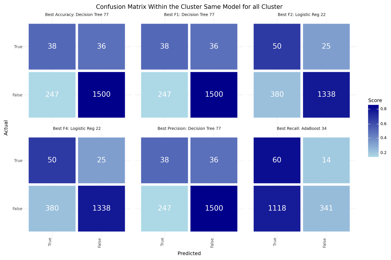
Confusion matrix - Best models for Cluster individual classification
Results for Best Model per Cluster
| Clustering | CID | Resampling | Scoring | Model | Precision | Recall | Accuracy | F1 | F2 | F4 | |
|---|---|---|---|---|---|---|---|---|---|---|---|
| 448 | AggloAF | 0 | Adasyn | f1 | Log Reg | 0.3333 | 0.7500 | 0.9759 | 0.4615 | 0.6000 | 0.6986 |
| 480 | AggloAF | 1 | Adasyn | f1 | Log Reg | 1.0000 | 1.0000 | 1.0000 | 1.0000 | 1.0000 | 1.0000 |
| 519 | AggloAF | 2 | Adasyn | recall | AdaBoost | 0.0900 | 0.8182 | 0.5550 | 0.1622 | 0.3125 | 0.5543 |
| 560 | AggloAF | 3 | None | f1 | Log Reg | 0.1887 | 0.6250 | 0.6231 | 0.2899 | 0.4274 | 0.5502 |
| 594 | AggloAF | 4 | None | f1 | Naive Bayes | 0.1176 | 0.3333 | 0.8927 | 0.1739 | 0.2439 | 0.3009 |
| 628 | AggloAF | 5 | None | recall | Log Reg | 0.1719 | 0.8462 | 0.6382 | 0.2857 | 0.4741 | 0.6875 |
| 666 | AggloAF | 6 | None | f2 | Naive Bayes | 0.1750 | 1.0000 | 0.2048 | 0.2979 | 0.5147 | 0.7829 |
| 687 | AggloAF | 7 | Adasyn | f4 | AdaBoost | 0.0741 | 0.6667 | 0.7719 | 0.1333 | 0.2564 | 0.4533 |
| 721 | AggloAF | 8 | None | f1 | Dec. Tree | 0.1667 | 0.5000 | 0.8717 | 0.2500 | 0.3571 | 0.4474 |
| 343 | DBSCANAF | 0 | None | recall | AdaBoost | 0.2174 | 1.0000 | 0.4375 | 0.3571 | 0.5814 | 0.8252 |
| 377 | DBSCANAF | 1 | None | f2 | Dec. Tree | 0.1042 | 0.5682 | 0.8227 | 0.1761 | 0.3005 | 0.4502 |
| 400 | DBSCANAF | 2 | None | f1 | Log Reg | 0.1887 | 0.6250 | 0.6231 | 0.2899 | 0.4274 | 0.5502 |
| 438 | DBSCANAF | 3 | None | recall | Naive Bayes | 0.2500 | 1.0000 | 0.3684 | 0.4000 | 0.6250 | 0.8500 |
| 21 | KMeanAF | 0 | None | recall | Dec. Tree | 0.0794 | 0.5000 | 0.7249 | 0.1370 | 0.2427 | 0.3812 |
| 32 | KMeanAF | 1 | Adasyn | f1 | Log Reg | 0.5000 | 1.0000 | 0.9961 | 0.6667 | 0.8333 | 0.9444 |
| 64 | KMeanAF | 2 | Adasyn | f1 | Log Reg | 0.2500 | 0.4286 | 0.9065 | 0.3158 | 0.3750 | 0.4113 |
| 113 | KMeanAF | 3 | None | f1 | Dec. Tree | 0.1875 | 0.8571 | 0.6747 | 0.3077 | 0.5000 | 0.7083 |
| 144 | KMeanAF | 4 | None | f1 | Log Reg | 0.0870 | 0.8571 | 0.5461 | 0.1579 | 0.3093 | 0.5635 |
| 160 | KMeanAF | 5 | Adasyn | f1 | Log Reg | 1.0000 | 1.0000 | 1.0000 | 1.0000 | 1.0000 | 1.0000 |
| 218 | KMeanAF | 6 | None | f2 | Naive Bayes | 0.1750 | 1.0000 | 0.2048 | 0.2979 | 0.5147 | 0.7829 |
| 243 | KMeanAF | 7 | None | f1 | AdaBoost | 0.1852 | 0.7143 | 0.8400 | 0.2941 | 0.4545 | 0.6115 |
| 274 | KMeanAF | 8 | None | f1 | Naive Bayes | 0.1818 | 0.4000 | 0.8909 | 0.2500 | 0.3226 | 0.3736 |
| 304 | KMeanAF | 9 | None | f1 | Log Reg | 0.1887 | 0.6250 | 0.6231 | 0.2899 | 0.4274 | 0.5502 |
| Clustering | CID | Resampling | Scoring | Model | F2 | True 1 | True 0 | False 1 | False 0 | |
|---|---|---|---|---|---|---|---|---|---|---|
| 448 | AggloAF | 0 | Adasyn | f1 | Log Reg | 0.6000 | 3 | 280 | 6 | 1 |
| 480 | AggloAF | 1 | Adasyn | f1 | Log Reg | 1.0000 | 0 | 451 | 0 | 0 |
| 519 | AggloAF | 2 | Adasyn | recall | AdaBoost | 0.3125 | 9 | 107 | 91 | 2 |
| 560 | AggloAF | 3 | None | f1 | Log Reg | 0.4274 | 10 | 71 | 43 | 6 |
| 594 | AggloAF | 4 | None | f1 | Naive Bayes | 0.2439 | 2 | 156 | 15 | 4 |
| 628 | AggloAF | 5 | None | recall | Log Reg | 0.4741 | 11 | 86 | 53 | 2 |
| 666 | AggloAF | 6 | None | f2 | Naive Bayes | 0.5147 | 14 | 3 | 66 | 0 |
| 687 | AggloAF | 7 | Adasyn | f4 | AdaBoost | 0.2564 | 2 | 86 | 25 | 1 |
| 721 | AggloAF | 8 | None | f1 | Dec. Tree | 0.3571 | 4 | 159 | 20 | 4 |
| 343 | DBSCANAF | 0 | None | recall | AdaBoost | 0.5814 | 10 | 18 | 36 | 0 |
| 377 | DBSCANAF | 1 | None | f2 | Dec. Tree | 0.3005 | 25 | 1061 | 215 | 19 |
| 400 | DBSCANAF | 2 | None | f1 | Log Reg | 0.4274 | 10 | 71 | 43 | 6 |
| 438 | DBSCANAF | 3 | None | recall | Naive Bayes | 0.6250 | 4 | 3 | 12 | 0 |
| 21 | KMeanAF | 0 | None | recall | Dec. Tree | 0.2427 | 5 | 161 | 58 | 5 |
| 32 | KMeanAF | 1 | Adasyn | f1 | Log Reg | 0.8333 | 1 | 253 | 1 | 0 |
| 64 | KMeanAF | 2 | Adasyn | f1 | Log Reg | 0.3750 | 3 | 123 | 9 | 4 |
| 113 | KMeanAF | 3 | None | f1 | Dec. Tree | 0.5000 | 6 | 50 | 26 | 1 |
| 144 | KMeanAF | 4 | None | f1 | Log Reg | 0.3093 | 6 | 71 | 63 | 1 |
| 160 | KMeanAF | 5 | Adasyn | f1 | Log Reg | 1.0000 | 0 | 501 | 0 | 0 |
| 218 | KMeanAF | 6 | None | f2 | Naive Bayes | 0.5147 | 14 | 3 | 66 | 0 |
| 243 | KMeanAF | 7 | None | f1 | AdaBoost | 0.4545 | 5 | 121 | 22 | 2 |
| 274 | KMeanAF | 8 | None | f1 | Naive Bayes | 0.3226 | 2 | 96 | 9 | 3 |
| 304 | KMeanAF | 9 | None | f1 | Log Reg | 0.4274 | 10 | 71 | 43 | 6 |
| Clustering | Precision | Recall | Accuracy | F1 | F2 | F4 | |
|---|---|---|---|---|---|---|---|
| 0 | AggloAF | 0.1471 | 0.7333 | 0.8109 | 0.2450 | 0.4080 | 0.5940 |
| 2 | KMeanAF | 0.1490 | 0.7027 | 0.8248 | 0.2459 | 0.4031 | 0.5766 |
| 1 | DBSCANAF | 0.1380 | 0.6622 | 0.7841 | 0.2284 | 0.3763 | 0.5413 |
| Clustering | F2 | True 1 | True 0 | False 1 | False 0 | |
|---|---|---|---|---|---|---|
| 0 | AggloAF | 0.4080 | 55 | 1399 | 319 | 20 |
| 2 | KMeanAF | 0.4031 | 52 | 1450 | 297 | 22 |
| 1 | DBSCANAF | 0.3763 | 49 | 1153 | 306 | 25 |
The best models depending on the scoring metric are shown below.
| Best Accuracy | Best Precision | Best Recall | Best F1 | Best F2 | Best F4 | |
|---|---|---|---|---|---|---|
| Model ID | 2 | 2 | 0 | 2 | 0 | 0 |
| Clustering | KMeanAF | KMeanAF | AggloAF | KMeanAF | AggloAF | AggloAF |
| Precision | 0.149 | 0.149 | 0.1471 | 0.149 | 0.1471 | 0.1471 |
| Recall | 0.7027 | 0.7027 | 0.7333 | 0.7027 | 0.7333 | 0.7333 |
| Accuracy | 0.8248 | 0.8248 | 0.8109 | 0.8248 | 0.8109 | 0.8109 |
| F1 | 0.2459 | 0.2459 | 0.245 | 0.2459 | 0.245 | 0.245 |
| F2 | 0.4031 | 0.4031 | 0.408 | 0.4031 | 0.408 | 0.408 |
| F4 | 0.5766 | 0.5766 | 0.594 | 0.5766 | 0.594 | 0.594 |
| True 1 | 52 | 52 | 55 | 52 | 55 | 55 |
| True 0 | 1450 | 1450 | 1399 | 1450 | 1399 | 1399 |
| False 1 | 297 | 297 | 319 | 297 | 319 | 319 |
| False 0 | 22 | 22 | 20 | 22 | 20 | 20 |
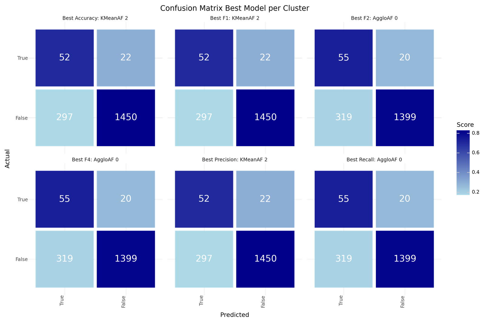
Confusion matrix - Best Models for for Best Model per Cluster
6. Dimensionality reduction - PCA and KPCA
Dimensionality reduction is crucial when working with high-dimensional datasets like the stroke dataset because it helps simplify the data, making it easier to visualize and analyze. High-dimensional data can be complex and computationally expensive to process, and it often contains redundant or irrelevant features that can obscure meaningful patterns. By reducing the number of dimensions, we can highlight the most important features that capture the majority of the data's variance, thus facilitating more efficient and insightful analysis. Reducing dimensions aids in visualizing the data, which is essential for understanding the underlying structure and relationships within the dataset. Visualizing the data in two dimensions can help identify clusters of patients with similar characteristics or risk profiles. This can provide valuable insights for developing targeted prevention and treatment strategies, ultimately improving patient outcomes. We will apply two widely used dimensionality reduction methods:
-
PCA : Principal Component Analysis and
-
KPCA : Kernel Function Principal Component Analysis.
PCA
Principal Component Analysis (PCA) is a widely used technique for dimensionality reduction that transforms the original high-dimensional data into a new set of uncorrelated variables called principal components. These principal components are linear combinations of the original features, ordered by the amount of variance they capture in the data. The first principal component captures the most variance, followed by the second, and so on. By selecting a subset of these components, we can reduce the dimensionality of the dataset while retaining most of its variability. PCA is particularly useful for identifying patterns and trends in the data, as well as for noise reduction and feature extraction.
In a first attempt to support vizualisation we will first scale the data and then run PCA to reduce to 2 Dimensions.
| count | mean | std | min | 25% | 50% | 75% | max | |
|---|---|---|---|---|---|---|---|---|
| gender | 5104.0 | 0.0 | 1.0 | -0.840 | -0.840 | -0.840 | 1.188 | 3.217 |
| age | 5104.0 | -0.0 | 1.0 | -1.910 | -0.807 | 0.077 | 0.785 | 1.714 |
| hypertension | 5104.0 | -0.0 | 1.0 | -0.328 | -0.328 | -0.328 | -0.328 | 3.051 |
| heart_disease | 5104.0 | 0.0 | 1.0 | -0.239 | -0.239 | -0.239 | -0.239 | 4.182 |
| ever_married | 5104.0 | -0.0 | 1.0 | -1.383 | -1.383 | 0.723 | 0.723 | 0.723 |
| work_type | 5104.0 | -0.0 | 1.0 | -1.988 | -0.153 | -0.153 | 0.764 | 1.681 |
| Residence_type | 5104.0 | 0.0 | 1.0 | -1.017 | -1.017 | 0.984 | 0.984 | 0.984 |
| smoking_status | 5104.0 | -0.0 | 1.0 | -1.286 | -1.286 | 0.581 | 0.581 | 1.515 |
| glucose_group | 5104.0 | 0.0 | 1.0 | -0.412 | -0.412 | -0.412 | -0.412 | 2.945 |
| bmi_group | 5104.0 | -0.0 | 1.0 | -2.129 | -1.079 | -0.030 | 1.020 | 1.020 |
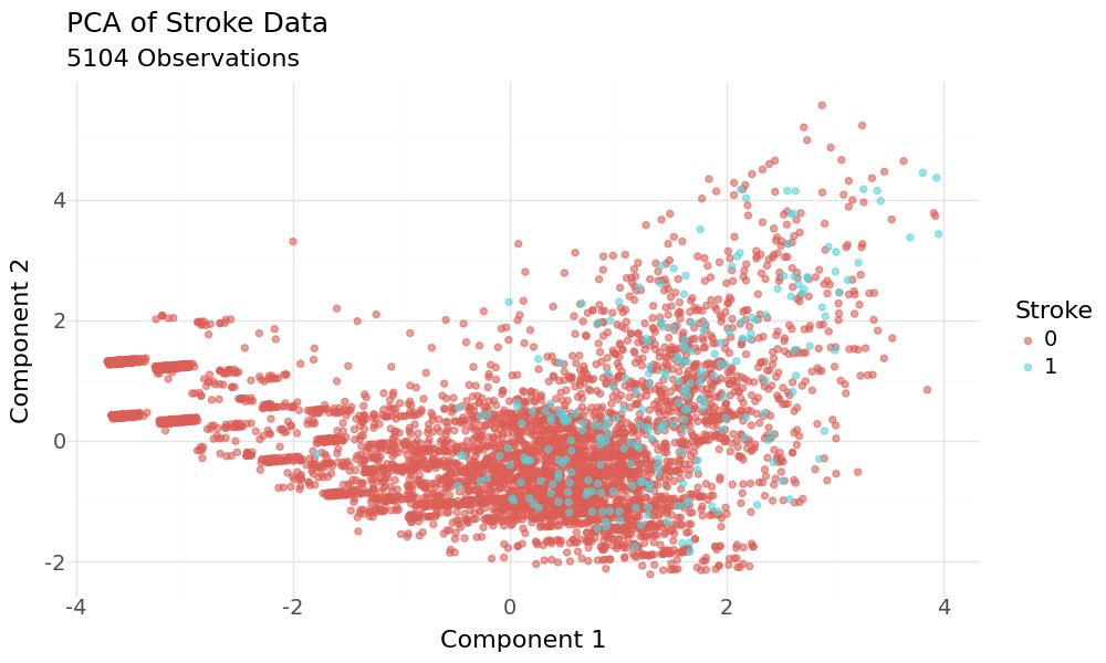
Scatterplot of 2D PCA principal components and target variable stroke as hue
The plot doesn't show good separation regarding the target variable. Also the cummulative explained variance ratio is not very good at 0.399.
| Principal Component | Explained Variance Ratio | Cumulative EVR | Eigenvalues | |
|---|---|---|---|---|
| 0 | PC1 | 0.274 | 0.274 | 2.738 |
| 1 | PC2 | 0.125 | 0.399 | 1.252 |
So we rerun PCA with the aim to explain 95% of the variance and plot the cummulative Variance.
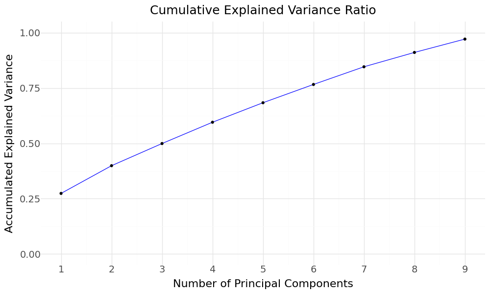
PCA Cummulative explained variance
We would require 9 components to explain 97% of the 10 features in our dataset.
[H]
10 1.2| Principal Component | Explained Variance Ratio | Cumulative EVR | Eigenvalues | |
|---|---|---|---|---|
| 0 | PC1 | 0.274 | 0.274 | 2.738 |
| 1 | PC2 | 0.125 | 0.399 | 1.252 |
| 2 | PC3 | 0.100 | 0.499 | 1.001 |
| 3 | PC4 | 0.096 | 0.595 | 0.962 |
| 4 | PC5 | 0.088 | 0.683 | 0.882 |
| 5 | PC6 | 0.082 | 0.766 | 0.825 |
| 6 | PC7 | 0.080 | 0.846 | 0.799 |
| 7 | PC8 | 0.065 | 0.911 | 0.648 |
| 8 | PC9 | 0.060 | 0.971 | 0.603 |
Now we try to fit classification models for the principal components as features. The results are listed below.
| Resampling | Scoring | Model | Precision | Recall | Accuracy | F1 | F2 | F4 | |
|---|---|---|---|---|---|---|---|---|---|
| 3 | Adasyn | f1 | AdaBoost | 0.114 | 0.784 | 0.696 | 0.199 | 0.361 | 0.583 |
| 0 | Adasyn | f1 | Logistic Regression | 0.115 | 0.743 | 0.711 | 0.199 | 0.355 | 0.562 |
| 8 | Adasyn | f2 | Logistic Regression | 0.115 | 0.743 | 0.711 | 0.199 | 0.355 | 0.562 |
| 4 | Adasyn | recall | Logistic Regression | 0.111 | 0.730 | 0.704 | 0.193 | 0.345 | 0.549 |
| 12 | Adasyn | f4 | Logistic Regression | 0.111 | 0.730 | 0.704 | 0.193 | 0.345 | 0.549 |
| 7 | Adasyn | recall | AdaBoost | 0.075 | 0.946 | 0.435 | 0.139 | 0.285 | 0.563 |
| 11 | Adasyn | f2 | AdaBoost | 0.075 | 0.946 | 0.435 | 0.139 | 0.285 | 0.563 |
| 15 | Adasyn | f4 | AdaBoost | 0.075 | 0.946 | 0.435 | 0.139 | 0.285 | 0.563 |
| Resampling | Scoring | Model | F2 | True 1 | True 0 | False 1 | False 0 | |
|---|---|---|---|---|---|---|---|---|
| 3 | Adasyn | f1 | AdaBoost | 0.361 | 58 | 1008 | 450 | 16 |
| 0 | Adasyn | f1 | Logistic Regression | 0.355 | 55 | 1034 | 424 | 19 |
| 8 | Adasyn | f2 | Logistic Regression | 0.355 | 55 | 1034 | 424 | 19 |
| 4 | Adasyn | recall | Logistic Regression | 0.345 | 54 | 1025 | 433 | 20 |
| 12 | Adasyn | f4 | Logistic Regression | 0.345 | 54 | 1025 | 433 | 20 |
| 7 | Adasyn | recall | AdaBoost | 0.285 | 70 | 597 | 861 | 4 |
| 11 | Adasyn | f2 | AdaBoost | 0.285 | 70 | 597 | 861 | 4 |
| 15 | Adasyn | f4 | AdaBoost | 0.285 | 70 | 597 | 861 | 4 |
The best models depending on the scoring metric are shown below.
| Best Accuracy | Best Precision | Best Recall | Best F1 | Best F2 | Best F4 | |
|---|---|---|---|---|---|---|
| Model ID | 0 | 0 | 7 | 3 | 3 | 3 |
| Resampling | Adasyn | Adasyn | Adasyn | Adasyn | Adasyn | Adasyn |
| Scoring | f1 | f1 | recall | f1 | f1 | f1 |
| Model | Logistic Reg | Logistic Reg | AdaBoost | AdaBoost | AdaBoost | AdaBoost |
| Precision | 0.115 | 0.115 | 0.075 | 0.114 | 0.114 | 0.114 |
| Recall | 0.743 | 0.743 | 0.946 | 0.784 | 0.784 | 0.784 |
| Accuracy | 0.711 | 0.711 | 0.435 | 0.696 | 0.696 | 0.696 |
| F1 | 0.199 | 0.199 | 0.139 | 0.199 | 0.199 | 0.199 |
| F2 | 0.355 | 0.355 | 0.285 | 0.361 | 0.361 | 0.361 |
| F4 | 0.562 | 0.562 | 0.563 | 0.583 | 0.583 | 0.583 |
| True 1 | 55 | 55 | 70 | 58 | 58 | 58 |
| True 0 | 1034 | 1034 | 597 | 1008 | 1008 | 1008 |
| False 1 | 424 | 424 | 861 | 450 | 450 | 450 |
| False 0 | 19 | 19 | 4 | 16 | 16 | 16 |
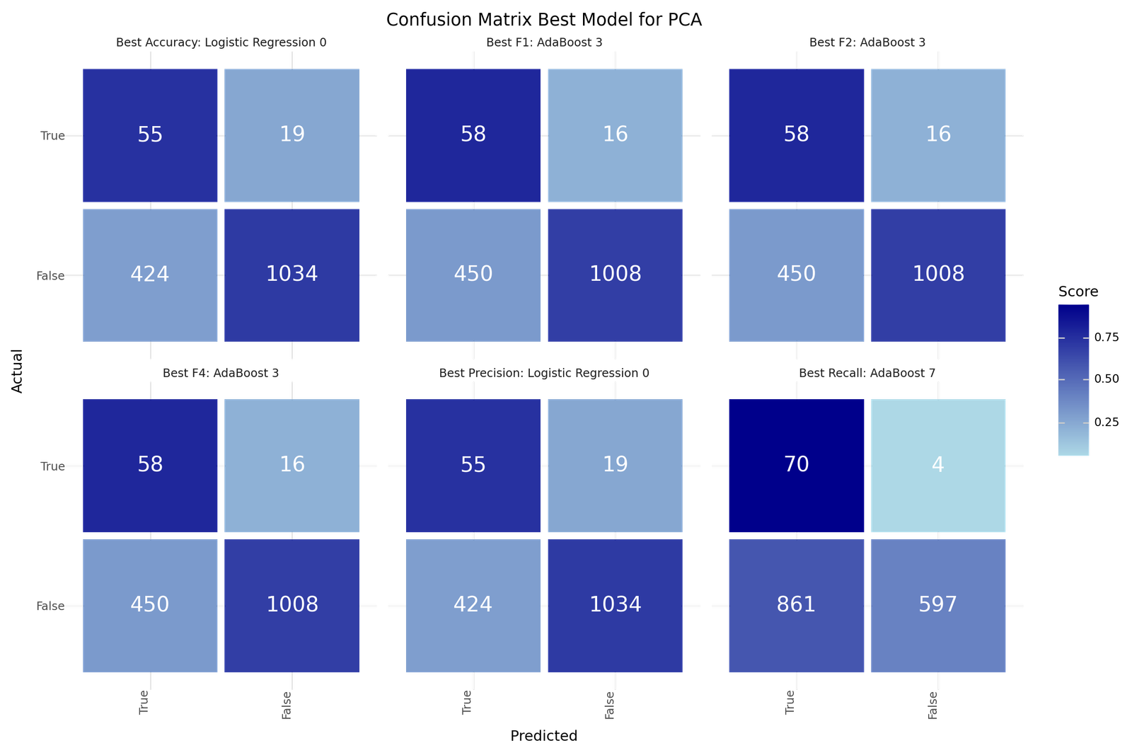
Confusion matrix Best models for PCA based classification
KPCA
Kernel PCA (KPCA) extends the traditional PCA method by using kernel functions to handle non-linear relationships in the data. While PCA is limited to linear transformations, KPCA projects the data into a higher-dimensional space using a kernel function, allowing it to capture complex, non-linear structures. The kernel function implicitly computes the principal components in this higher-dimensional space without the need to explicitly perform the transformation, making it computationally efficient. KPCA is especially useful when the data has intricate non-linear patterns that cannot be captured by linear methods like PCA. It provides a more flexible approach to dimensionality reduction, enabling better feature extraction and improved performance of machine learning algorithms on complex datasets.
As with PCA we will first scale the data and then run PCA to reduce to 2 Dimensions.
| count | mean | std | min | 25% | 50% | 75% | max | |
|---|---|---|---|---|---|---|---|---|
| gender | 5104.0 | 0.0 | 1.0 | -0.840 | -0.840 | -0.840 | 1.188 | 3.217 |
| age | 5104.0 | -0.0 | 1.0 | -1.910 | -0.807 | 0.077 | 0.785 | 1.714 |
| hypertension | 5104.0 | -0.0 | 1.0 | -0.328 | -0.328 | -0.328 | -0.328 | 3.051 |
| heart_disease | 5104.0 | 0.0 | 1.0 | -0.239 | -0.239 | -0.239 | -0.239 | 4.182 |
| ever_married | 5104.0 | -0.0 | 1.0 | -1.383 | -1.383 | 0.723 | 0.723 | 0.723 |
| work_type | 5104.0 | -0.0 | 1.0 | -1.988 | -0.153 | -0.153 | 0.764 | 1.681 |
| Residence_type | 5104.0 | 0.0 | 1.0 | -1.017 | -1.017 | 0.984 | 0.984 | 0.984 |
| smoking_status | 5104.0 | -0.0 | 1.0 | -1.286 | -1.286 | 0.581 | 0.581 | 1.515 |
| glucose_group | 5104.0 | 0.0 | 1.0 | -0.412 | -0.412 | -0.412 | -0.412 | 2.945 |
| bmi_group | 5104.0 | -0.0 | 1.0 | -2.129 | -1.079 | -0.030 | 1.020 | 1.020 |
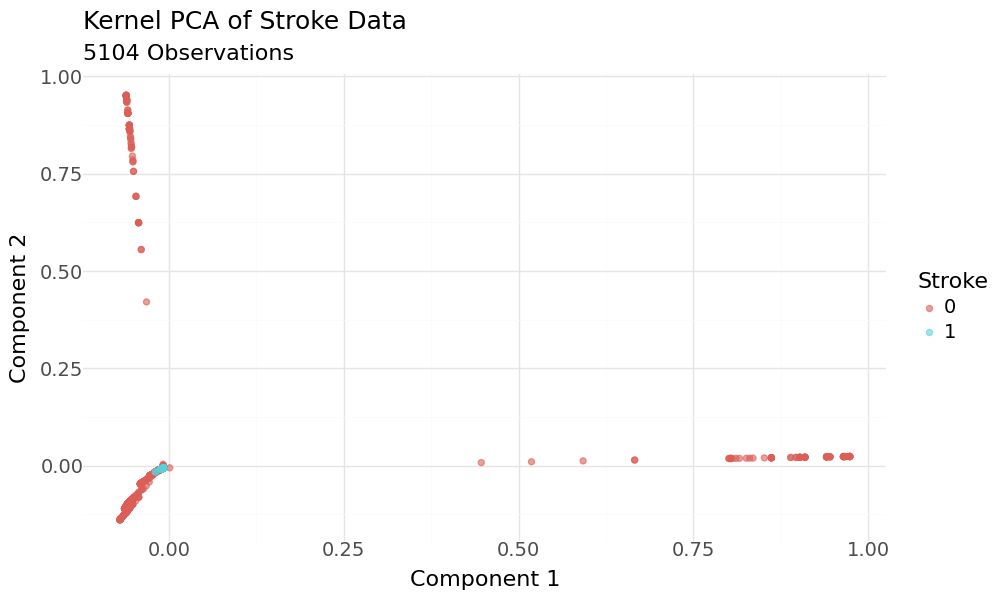
Scatterplot of 2D KPCA principal components and target variable stroke as hue
The plot appears to show good separation regarding the target variable. When we zoom into the range of the target variable and have a closer look, we can see that the classes are hardly separated.
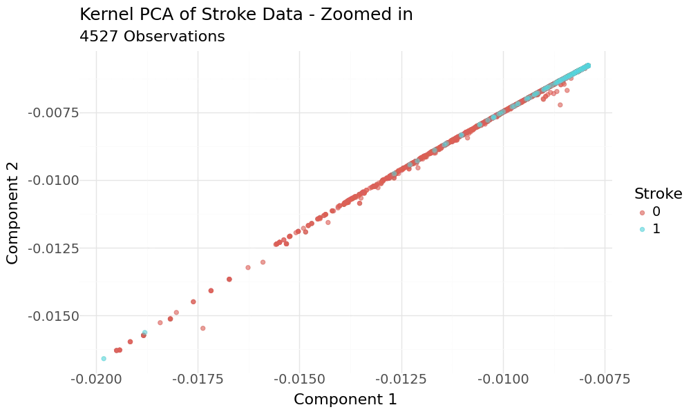
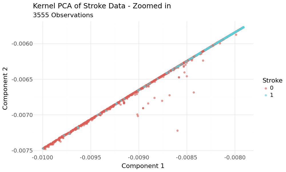
Zoomed in Scatterplots of 2D KPCA principal components and target variable stroke as hue
When we rerun KPCA without specifying the number of components, we can then see how much variance is explained by each principal component, if we take a look at the magnitude of their respective eigenvalues.
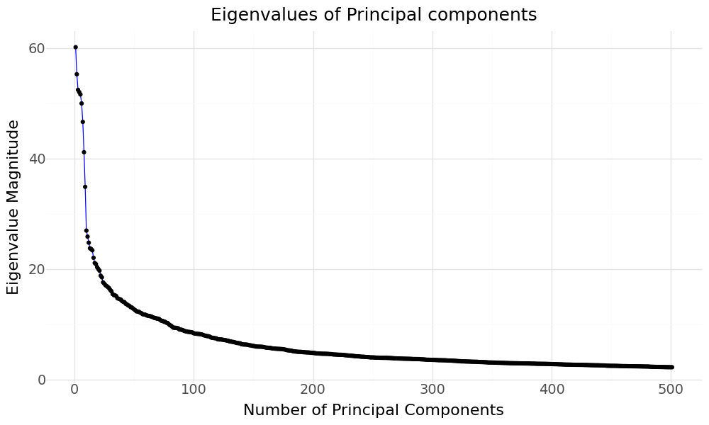
Eigenvalues of KPCA Principal Components
We can try to evaluate the Kernel PCA results with applying our different classifcation models and their performance using the principal components as features and the stroke variable as target. We will evaluate for 20,40 and 60 principal components.
| KPC | Resampling | Scoring | Model | Precision | Recall | Accuracy | F1 | F2 | F4 | |
|---|---|---|---|---|---|---|---|---|---|---|
| 3 | 20 | Adasyn | f1 | AdaBoost | 0.1231 | 0.7703 | 0.7239 | 0.2123 | 0.3755 | 0.5883 |
| 35 | 40 | Adasyn | f1 | AdaBoost | 0.1223 | 0.7568 | 0.7258 | 0.2105 | 0.3714 | 0.5798 |
| 32 | 40 | Adasyn | f1 | Logistic Regression | 0.1225 | 0.7432 | 0.7304 | 0.2103 | 0.3691 | 0.5726 |
| 36 | 40 | Adasyn | recall | Logistic Regression | 0.1225 | 0.7432 | 0.7304 | 0.2103 | 0.3691 | 0.5726 |
| 40 | 40 | Adasyn | f2 | Logistic Regression | 0.1225 | 0.7432 | 0.7304 | 0.2103 | 0.3691 | 0.5726 |
| 44 | 40 | Adasyn | f4 | Logistic Regression | 0.1225 | 0.7432 | 0.7304 | 0.2103 | 0.3691 | 0.5726 |
| 0 | 20 | Adasyn | f1 | Logistic Regression | 0.1204 | 0.7432 | 0.7252 | 0.2072 | 0.3652 | 0.5698 |
| 4 | 20 | Adasyn | recall | Logistic Regression | 0.1198 | 0.7432 | 0.7239 | 0.2064 | 0.3642 | 0.5691 |
| 8 | 20 | Adasyn | f2 | Logistic Regression | 0.1198 | 0.7432 | 0.7239 | 0.2064 | 0.3642 | 0.5691 |
| 12 | 20 | Adasyn | f4 | Logistic Regression | 0.1198 | 0.7432 | 0.7239 | 0.2064 | 0.3642 | 0.5691 |
| 68 | 60 | Adasyn | recall | Logistic Regression | 0.1189 | 0.7297 | 0.7258 | 0.2045 | 0.3600 | 0.5604 |
| 64 | 60 | Adasyn | f1 | Logistic Regression | 0.1189 | 0.7297 | 0.7258 | 0.2045 | 0.3600 | 0.5604 |
| 72 | 60 | Adasyn | f2 | Logistic Regression | 0.1189 | 0.7297 | 0.7258 | 0.2045 | 0.3600 | 0.5604 |
| 76 | 60 | Adasyn | f4 | Logistic Regression | 0.1189 | 0.7297 | 0.7258 | 0.2045 | 0.3600 | 0.5604 |
| 60 | 40 | TomekLinks | f4 | Logistic Regression | 0.1182 | 0.7297 | 0.7239 | 0.2034 | 0.3586 | 0.5594 |
| 52 | 40 | TomekLinks | recall | Logistic Regression | 0.1182 | 0.7297 | 0.7239 | 0.2034 | 0.3586 | 0.5594 |
| 56 | 40 | TomekLinks | f2 | Logistic Regression | 0.1182 | 0.7297 | 0.7239 | 0.2034 | 0.3586 | 0.5594 |
| 48 | 40 | TomekLinks | f1 | Logistic Regression | 0.1182 | 0.7297 | 0.7239 | 0.2034 | 0.3586 | 0.5594 |
| 16 | 20 | TomekLinks | f1 | Logistic Regression | 0.1048 | 0.8243 | 0.6514 | 0.1860 | 0.3474 | 0.5872 |
| 43 | 40 | Adasyn | f2 | AdaBoost | 0.0870 | 0.8514 | 0.5614 | 0.1579 | 0.3088 | 0.5613 |
| 181 | 60 | TomekLinks | recall | Decision Tree | 0.0832 | 0.7432 | 0.5920 | 0.1497 | 0.2874 | 0.5068 |
| 131 | 40 | Adasyn | f1 | AdaBoost | 0.0804 | 0.7703 | 0.5633 | 0.1456 | 0.2836 | 0.5119 |
| 103 | 20 | Adasyn | recall | AdaBoost | 0.0791 | 0.7703 | 0.5555 | 0.1434 | 0.2802 | 0.5087 |
| 111 | 20 | Adasyn | f4 | AdaBoost | 0.0791 | 0.7703 | 0.5555 | 0.1434 | 0.2802 | 0.5087 |
| 107 | 20 | Adasyn | f2 | AdaBoost | 0.0782 | 0.7703 | 0.5503 | 0.1420 | 0.2780 | 0.5065 |
| 163 | 60 | Adasyn | f1 | AdaBoost | 0.0794 | 0.7297 | 0.5783 | 0.1432 | 0.2766 | 0.4925 |
| 99 | 20 | Adasyn | f1 | AdaBoost | 0.0779 | 0.7568 | 0.5555 | 0.1412 | 0.2759 | 0.5003 |
| KPC | Resampling | Scoring | Model | F2 | True 1 | True 0 | False 1 | False 0 | |
|---|---|---|---|---|---|---|---|---|---|
| 3 | 20 | Adasyn | f1 | AdaBoost | 0.3755 | 57 | 1052 | 406 | 17 |
| 35 | 40 | Adasyn | f1 | AdaBoost | 0.3714 | 56 | 1056 | 402 | 18 |
| 32 | 40 | Adasyn | f1 | Logistic Regression | 0.3691 | 55 | 1064 | 394 | 19 |
| 36 | 40 | Adasyn | recall | Logistic Regression | 0.3691 | 55 | 1064 | 394 | 19 |
| 40 | 40 | Adasyn | f2 | Logistic Regression | 0.3691 | 55 | 1064 | 394 | 19 |
| 44 | 40 | Adasyn | f4 | Logistic Regression | 0.3691 | 55 | 1064 | 394 | 19 |
| 0 | 20 | Adasyn | f1 | Logistic Regression | 0.3652 | 55 | 1056 | 402 | 19 |
| 4 | 20 | Adasyn | recall | Logistic Regression | 0.3642 | 55 | 1054 | 404 | 19 |
| 8 | 20 | Adasyn | f2 | Logistic Regression | 0.3642 | 55 | 1054 | 404 | 19 |
| 12 | 20 | Adasyn | f4 | Logistic Regression | 0.3642 | 55 | 1054 | 404 | 19 |
| 68 | 60 | Adasyn | recall | Logistic Regression | 0.3600 | 54 | 1058 | 400 | 20 |
| 64 | 60 | Adasyn | f1 | Logistic Regression | 0.3600 | 54 | 1058 | 400 | 20 |
| 72 | 60 | Adasyn | f2 | Logistic Regression | 0.3600 | 54 | 1058 | 400 | 20 |
| 76 | 60 | Adasyn | f4 | Logistic Regression | 0.3600 | 54 | 1058 | 400 | 20 |
| 60 | 40 | TomekLinks | f4 | Logistic Regression | 0.3586 | 54 | 1055 | 403 | 20 |
| 52 | 40 | TomekLinks | recall | Logistic Regression | 0.3586 | 54 | 1055 | 403 | 20 |
| 56 | 40 | TomekLinks | f2 | Logistic Regression | 0.3586 | 54 | 1055 | 403 | 20 |
| 48 | 40 | TomekLinks | f1 | Logistic Regression | 0.3586 | 54 | 1055 | 403 | 20 |
| 16 | 20 | TomekLinks | f1 | Logistic Regression | 0.3474 | 61 | 937 | 521 | 13 |
| 43 | 40 | Adasyn | f2 | AdaBoost | 0.3088 | 63 | 797 | 661 | 11 |
| 181 | 60 | TomekLinks | recall | Decision Tree | 0.2874 | 55 | 852 | 606 | 19 |
| 131 | 40 | Adasyn | f1 | AdaBoost | 0.2836 | 57 | 806 | 652 | 17 |
| 103 | 20 | Adasyn | recall | AdaBoost | 0.2802 | 57 | 794 | 664 | 17 |
| 111 | 20 | Adasyn | f4 | AdaBoost | 0.2802 | 57 | 794 | 664 | 17 |
| 107 | 20 | Adasyn | f2 | AdaBoost | 0.2780 | 57 | 786 | 672 | 17 |
| 163 | 60 | Adasyn | f1 | AdaBoost | 0.2766 | 54 | 832 | 626 | 20 |
| 99 | 20 | Adasyn | f1 | AdaBoost | 0.2759 | 56 | 795 | 663 | 18 |
The best models depending on the scoring metric are shown below.
| Best Accuracy | Best Precision | Best Recall | Best F1 | Best F2 | Best F4 | |
|---|---|---|---|---|---|---|
| Model ID | 32 | 3 | 43 | 3 | 3 | 3 |
| KPC | 40 | 20 | 40 | 20 | 20 | 20 |
| Resampling | Adasyn | Adasyn | Adasyn | Adasyn | Adasyn | Adasyn |
| Scoring | f1 | f1 | f2 | f1 | f1 | f1 |
| Model | Logistic Reg | AdaBoost | AdaBoost | AdaBoost | AdaBoost | AdaBoost |
| Precision | 0.1225 | 0.1231 | 0.087 | 0.1231 | 0.1231 | 0.1231 |
| Recall | 0.7432 | 0.7703 | 0.8514 | 0.7703 | 0.7703 | 0.7703 |
| Accuracy | 0.7304 | 0.7239 | 0.5614 | 0.7239 | 0.7239 | 0.7239 |
| F1 | 0.2103 | 0.2123 | 0.1579 | 0.2123 | 0.2123 | 0.2123 |
| F2 | 0.3691 | 0.3755 | 0.3088 | 0.3755 | 0.3755 | 0.3755 |
| F4 | 0.5726 | 0.5883 | 0.5613 | 0.5883 | 0.5883 | 0.5883 |
| True 1 | 55 | 57 | 63 | 57 | 57 | 57 |
| True 0 | 1064 | 1052 | 797 | 1052 | 1052 | 1052 |
| False 1 | 394 | 406 | 661 | 406 | 406 | 406 |
| False 0 | 19 | 17 | 11 | 17 | 17 | 17 |
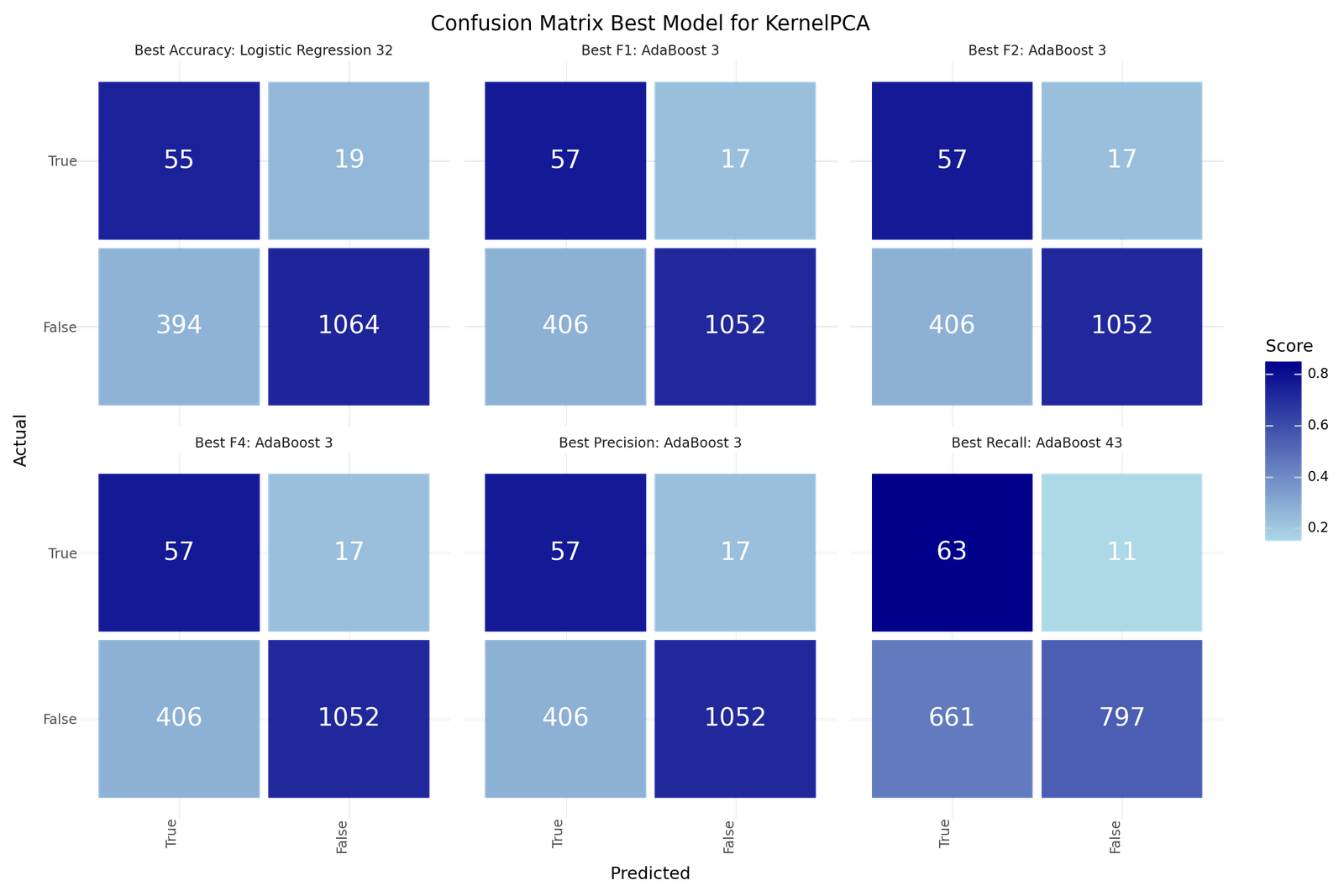
Confusion matrix - Best model for KPCA based classification
7. Recommended Model
After training and evaluating the models, it is hard to identify a single best model as it is highly depending on the preference on how you value the misclassification of a stroke patient. We did not gain huge improvements with the unsupervised leaning approaches but could identify slight improvement in the F4 score for Cluster based classification. Dimensionality Reduction did not result in improved results compared to the base models. Based on our performance metric we can propose two models as promising. The best F2 value was achieved with the base classification only AdaBoost model number 19 with under-sampling. The best F4 value was realized by applying AdaBoost model number 63 with under-sampling and enriching the classification with the resulting cluster labels from the DBSCAN clustering. Both models could be a good starting point for further evaluation. Below you can find the Confusion Matrix for both models.
Best F2 Score
| Model 19 - AdaBoost | |
|---|---|
| Resampling | TomekLinks |
| Scoring | f1 |
| Model | AdaBoost |
| Precision | 0.167192 |
| Recall | 0.716216 |
| Accuracy | 0.813969 |
| F1 | 0.2711 |
| F2 | 0.4323 |
| F4 | 0.600266 |
| True 1 | 53 |
| True 0 | 1194 |
| False 1 | 264 |
| False 0 | 21 |
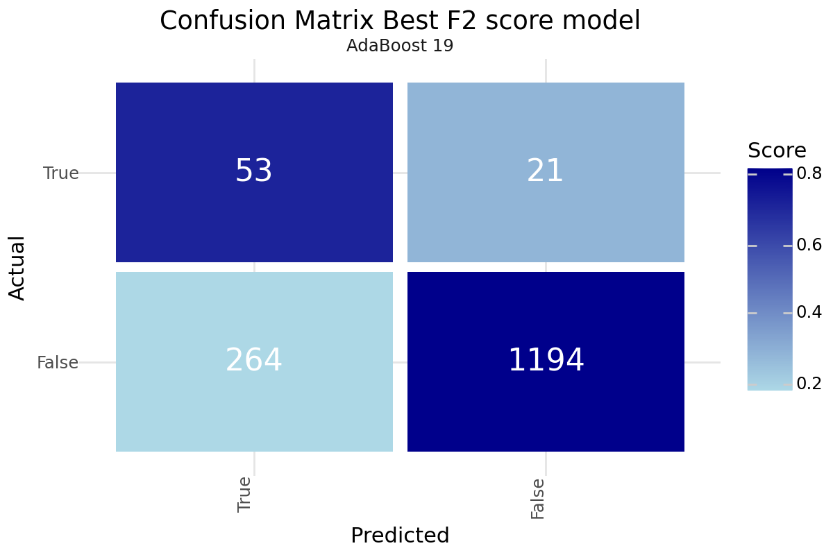
Confusion matrix Best F2 Score - AdaBoost Base model 19
Best F4 Score
| Model 63 - AdaBoost DBSCAN | |
|---|---|
| Clustering | DBSCANAF |
| Resampling | TomekLinks |
| Scoring | f4 |
| Model | AdaBoost |
| Precision | 0.10559 |
| Recall | 0.918919 |
| Accuracy | 0.619856 |
| F1 | 0.189415 |
| F2 | 0.361702 |
| F4 | 0.632385 |
| True 1 | 68 |
| True 0 | 881 |
| False 1 | 576 |
| False 0 | 6 |
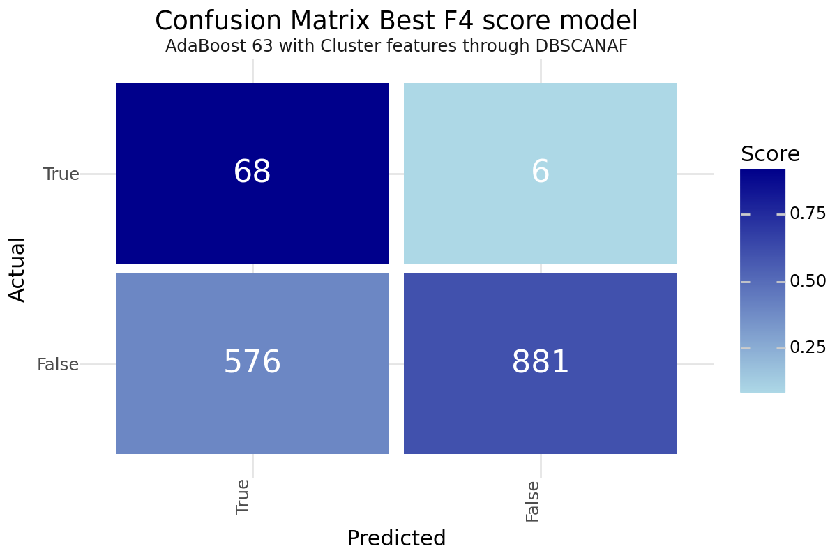
Confusion matrix Best F4 Score - AdaBoost DBSCAN Cluster model 63
8. Key Findings and Insights
The analysis of the stroke prediction model has revealed several critical factors that significantly influence the likelihood of stroke in patients. Understanding these drivers allows for better-targeted interventions and more effective prevention strategies. However, to further enhance the accuracy and reliability of the model, additional data and features are essential.
Main Drivers influencing Stroke Risk
-
Age: Older patients have a higher risk of stroke. This finding underscores the importance of age-related health monitoring and interventions, as the likelihood of experiencing a stroke increases with age, necessitating enhanced medical vigilance for the elderly.
-
Hypertension: Presence of hypertension increases stroke risk. Hypertension, or high blood pressure, is a well-established risk factor for stroke, emphasizing the need for strict blood pressure control through medication, lifestyle changes, and regular monitoring.
-
Heart Disease: Patients with heart disease are more likely to experience a stroke. The strong correlation between cardiovascular conditions and stroke highlights the necessity for comprehensive care plans that address both heart disease management and stroke prevention.
-
Average Glucose Level: Higher average glucose levels are associated with Diabetes and increase stroke risk. Elevated glucose levels indicate poor diabetes control, which can lead to vascular damage and increased stroke risk, highlighting the importance of maintaining optimal glucose levels through diet, exercise, and medication adherence.
Insights
-
Preventive Measures: Targeted interventions for patients with hypertension and heart disease could reduce stroke incidence. Implementing comprehensive care plans that include lifestyle modifications, medication adherence, and regular health check-ups is crucial for mitigating stroke risk in these high-risk populations.
-
Public Health Strategies: Programs aimed at managing blood glucose levels and promoting healthy aging could be beneficial. Public health initiatives should focus on widespread screening for diabetes and hypertension, coupled with campaigns that encourage physical activity, healthy eating, and smoking cessation to reduce stroke risk at a population level.
-
Holistic Health Approach: Adopting a holistic approach that considers the interplay between various risk factors can enhance stroke prevention efforts. By addressing lifestyle factors such as diet, exercise, and stress management, healthcare providers can simultaneously mitigate risks associated with hypertension, heart disease, and diabetes, leading to better overall health outcomes.
-
Technology and Monitoring: Leveraging technology, such as wearable devices and telemedicine, can aid in the continuous monitoring of at-risk individuals. These technologies provide real-time data on blood pressure, glucose levels, and heart rate, allowing for timely interventions and personalized care plans that can significantly reduce stroke risk.
-
Education and Awareness: Raising awareness about the risk factors and preventive measures for stroke is crucial. Public health campaigns and educational programs should aim to inform individuals about the importance of regular health screenings, recognizing early symptoms of stroke, and seeking immediate medical attention, empowering them to take proactive steps towards stroke prevention.
Future Directions
To further improve the understanding and prediction of stroke risk, it is imperative to gather more comprehensive data and incorporate additional features into the model. Including a wider range of demographic, genetic, and lifestyle factors can provide a more nuanced view of stroke risk. Additionally, longitudinal data tracking patients over time could offer insights into how risk factors evolve and interact. By expanding the dataset and refining the features used, we can develop more accurate and robust models that enhance our ability to prevent and manage stroke.
9. Suggestions for Next Steps
-
Feature Enhancement: Incorporate additional health-related features, such as cholesterol levels, physical activity, and diet, to improve the model's predictive performance. Including more comprehensive lifestyle and biometric data can help create a more accurate and holistic risk assessment for stroke.
-
Longitudinal Data: Utilize longitudinal data to track changes in patient health over time, which can provide deeper insights into the progression and interaction of risk factors. Longitudinal studies allow for the observation of how individual risk profiles evolve, leading to more precise and personalized predictions.
-
Assessment of Existing Studies and Scores: Evaluate and integrate findings from established studies and scoring systems, such as the Framingham Heart Study and the CHA₂DS₂-VASc score, which are widely used for predicting cardiovascular and stroke risk. Comparing our model's performance with these well-regarded benchmarks can provide validation and highlight areas for improvement. Additionally, exploring datasets from these studies can offer valuable insights and potential features to enhance our model.
-
Collaborative Research: Engage in collaborative research with other institutions and researchers to leverage a broader range of expertise and datasets. By pooling resources and knowledge, we can develop more robust and generalizable models that are applicable across diverse populations.
-
Validation Across Diverse Populations: Test and validate the model across different demographic and geographic populations to ensure its applicability and reliability. Understanding how the model performs in various contexts can help identify any biases or limitations, leading to more equitable and effective stroke risk prediction tools.
-
Model Re-evaluation: Regularly update and re-evaluate the model as new data becomes available to ensure its continued relevance and accuracy. Incorporating the latest research findings and medical advancements will help maintain the model's effectiveness in predicting stroke risk.