Stroke Prediction Analysis - Regression, Tree and Boosting Models with Regulation and Resampling
Summary
The primary objective of this analysis is to develop a predictive model for stroke risk using various health and demographic attributes, focusing on maximizing recall to minimize missed stroke cases. The dataset, sourced from Kaggle, contains information on 5,110 patients with attributes such as age, gender, hypertension, heart disease, and smoking status. Data exploration revealed age, hypertension, and heart disease as significant predictors of stroke risk. Various classification models were evaluated, with the AdaBoost model showing the best overall performance in terms of balancing true and false positives. The analysis recommends incorporating additional health-related features and using longitudinal data to improve model accuracy. Future work should also focus on validating the model across diverse populations and regularly updating it with new data to maintain its relevance and accuracy.
1. Main Objective of the Analysis
The primary objective of this analysis is to build a predictive model focused on predicting the likelihood of stroke in patients based on various health and demographic attributes. The objective for finding the best prediction is to maximize accuracy in terms of recall whilst not classifying too many cases wrongly as stroke risk. The true cost of misclassifying a patient at stroke risk as healthy outweighs the cost of misclassifying a healthy patient as at risk for stroke. The analysis aims at providing insights for stroke risk classification to allow:
- Early Identification: Helping healthcare providers identify individuals at higher risk of stroke for timely intervention.
- Resource Allocation: Assisting in the efficient allocation of medical resources to those most in need.
- Preventive Measures: Providing insights for developing targeted preventive measures to reduce the incidence of strokes.
2. Dataset Description
Dataset Overview
The Stroke Prediction dataset is available at Kaggle (URL : https://www.kaggle.com/fedesoriano/stroke-prediction-dataset) and contains data on patients, including their medical and demographic attributes.
Attributes
| Attribute | Description |
|---|---|
| id | Unique identifier for each patient. |
| gender | Gender of the patient (Male, Female, Other). |
| age | Age of the patient. |
| hypertension | Whether the patient has hypertension (0: No, 1: Yes). |
| heart_disease | Whether the patient has heart disease (0: No, 1: Yes). |
| ever_married | Marital status of the patient (No, Yes). |
| work_type | Type of occupation (children, Govt_job, Never_worked, Private, Self-employed). |
| residence_type | Type of residence (Rural, Urban). |
| avg_glucose_level | Average glucose level in the blood. |
| bmi | Body mass index. |
| smoking_status | Smoking status (formerly smoked, never smoked, smokes, Unknown). |
| stroke | Target variable indicating whether the patient had a stroke (0: No, 1: Yes). |
-
Number of Instances: 5,110
-
Number of Features: 11
-
Target Variable:
stroke(0: No Stroke, 1: Stroke)
Analysis Approach
The analysis aims to:
- Explore and visualize the data to understand the distribution of attributes and identify any missing or anomalous values.
- Engineer features and prepare the data for modeling.
- Train multiple classifier models to predict stroke risk and evaluate the performance of the models.
- Identify the best-performing model based on support for stroke risk management.
- Provide recommendations for next steps and further optimization.
3. Data Exploration and Cleaning
Data Exploration
Besides the id the dataset includes ten features as listed above plus the target variable stroke . There are three numerical features: age, avg_glucose_level and bmi. The remaining seven features are all categorical.
Out of the 5,110 observations in the dataset, 4861 were observed with no stroke and 249 patients had a stroke. The dataset could be classified as not balanced, which has to be addressed before model training.
The variables of the dataset and the distribution of the target variable are shown below.
| count | unique | top | freq | mean | std | min | 25% | 50% | 75% | max | |
|---|---|---|---|---|---|---|---|---|---|---|---|
| gender | 5110 | 3 | Female | 2994 | NaN | NaN | NaN | NaN | NaN | NaN | NaN |
| age | 5110.0 | NaN | NaN | NaN | 43.23 | 22.61 | 0.08 | 25.0 | 45.0 | 61.0 | 82.0 |
| hypertension | 5110.0 | NaN | NaN | NaN | 0.1 | 0.3 | 0.0 | 0.0 | 0.0 | 0.0 | 1.0 |
| heart_disease | 5110.0 | NaN | NaN | NaN | 0.05 | 0.23 | 0.0 | 0.0 | 0.0 | 0.0 | 1.0 |
| ever_married | 5110 | 2 | Yes | 3353 | NaN | NaN | NaN | NaN | NaN | NaN | NaN |
| work_type | 5110 | 5 | Private | 2925 | NaN | NaN | NaN | NaN | NaN | NaN | NaN |
| Residence_type | 5110 | 2 | Urban | 2596 | NaN | NaN | NaN | NaN | NaN | NaN | NaN |
| avg_glucose_level | 5110.0 | NaN | NaN | NaN | 106.15 | 45.28 | 55.12 | 77.24 | 91.88 | 114.09 | 271.74 |
| bmi | 4909.0 | NaN | NaN | NaN | 28.89 | 7.85 | 10.3 | 23.5 | 28.1 | 33.1 | 97.6 |
| smoking_status | 5110 | 4 | never smoked | 1892 | NaN | NaN | NaN | NaN | NaN | NaN | NaN |
| stroke | 5110.0 | NaN | NaN | NaN | 0.05 | 0.22 | 0.0 | 0.0 | 0.0 | 0.0 | 1.0 |
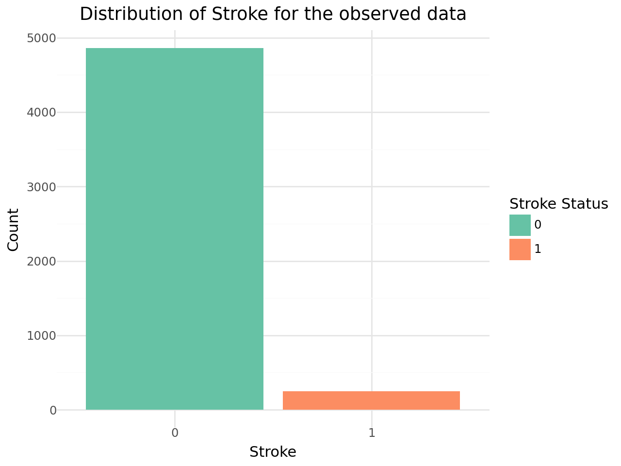
Distribution of stroke cases in the dataset
To analyze distribution and correlation of the data we prepared a set of 4 plots for each of the variables despending on the type as follows:
-
Numerical Variables: The overall distribution of the variable, the distribution of the variable for non stroke observations, the distribution of the variable for stroke observations and the density distribution separated by stroke cases.
-
Categorical Variables: The overall distribution of the variable, the distribution of the variable for non stroke observations, the distribution of the variable for stroke observations and the distribution of stroke cases within the groups of the categorical variable.
The distribution of the target variable is shown below.
Numerical Variables
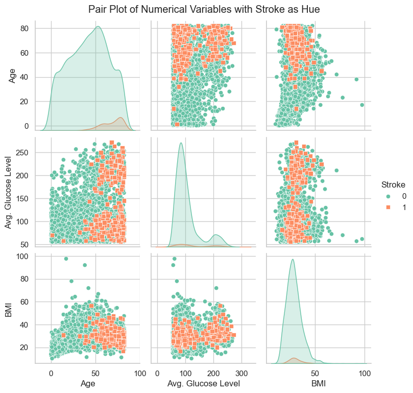
The graphs for the three numerical variables are shown below. There isn't a meaningful correlation visible for BMI or the Average Glucose Level. In contrast Age shows a fairly strong dependency with the target variable.
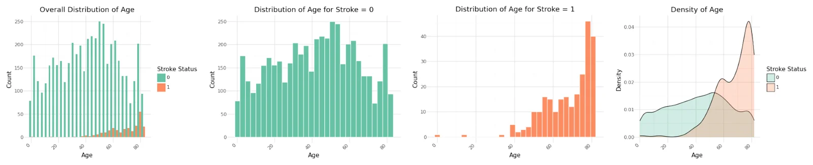
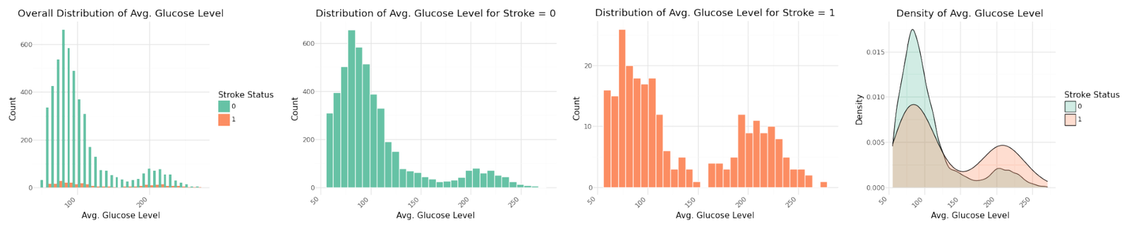
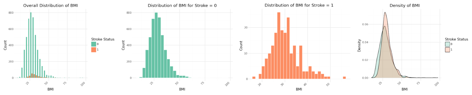
Distribution of numerical variables
Stroke cases plotted versus Age show to be not equally distributed. The reported stroke cases can be more often found with increasing age. Body Mass Index and Average Glucose level do not show an obvious influence on stroke. The observation is confirmed in the pairplot below.
Pairplot of numerical variable
As seen before here isn't a meaningful correlation visible for BMI or the Average Glucose Level, but Age shows a fairly strong left skew against the target variable.
Categorical Variables
The distribution of the seven categorical variables are shown below.
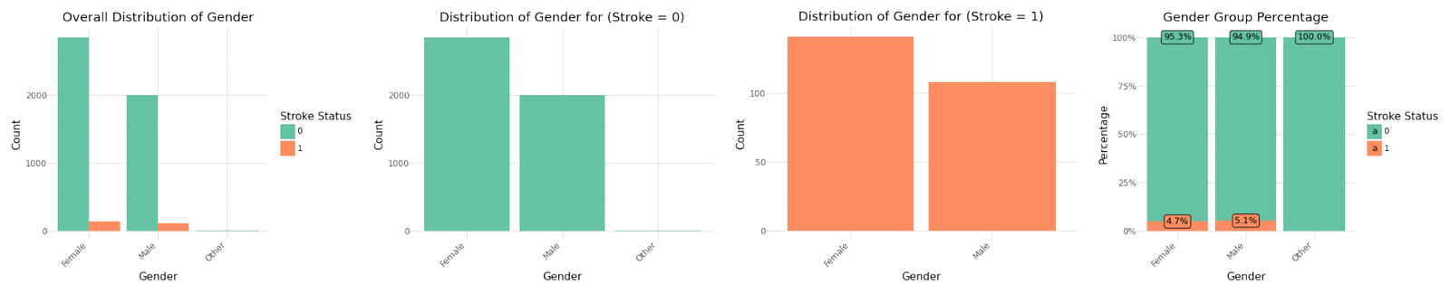
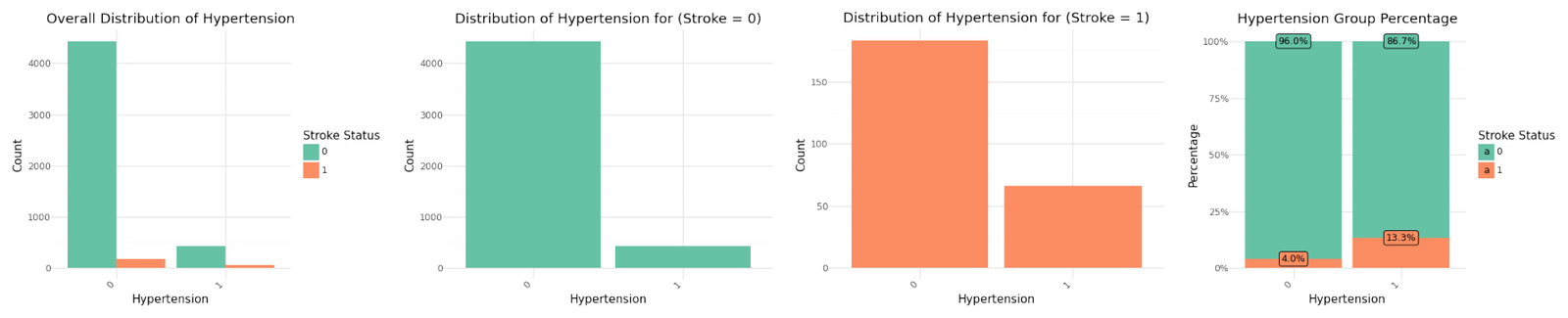
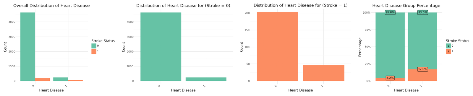
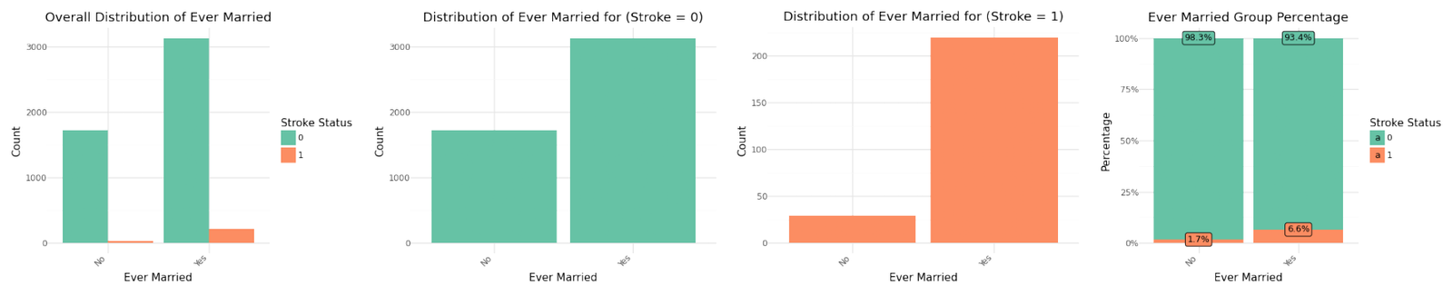
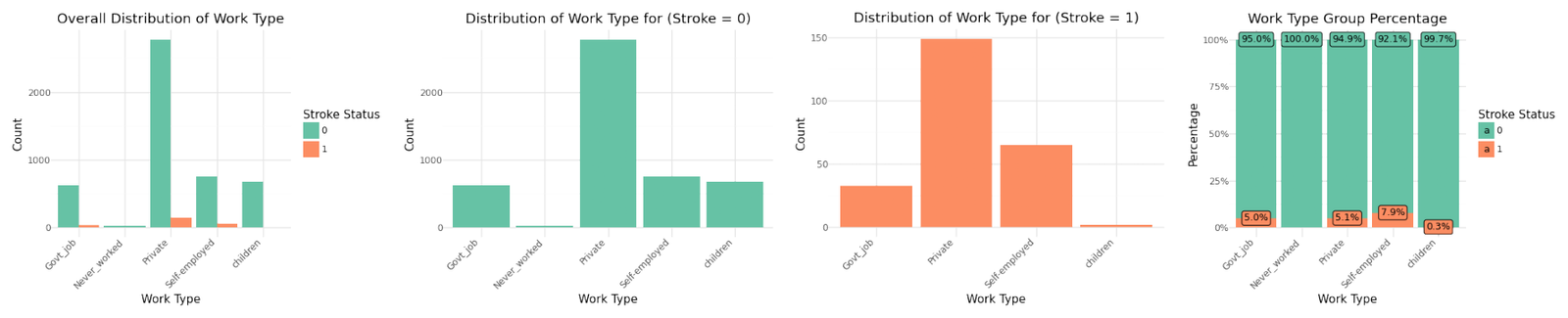
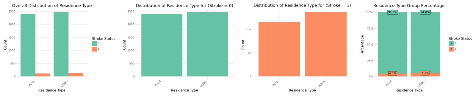
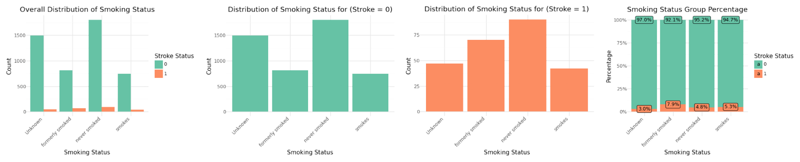
Distribution of categorical variables
If we analyze the group percentages and compare the distributions of the variables for stroke and non stroke cases we can identify Hypertension, Heat Disease and the Married Status as potential influence for stroke cases. We will analyze the correlation further below.
Correlation Analysis
We can pairplot the entire dataset after after coding and adding some noise to categorical variables for better illustration.
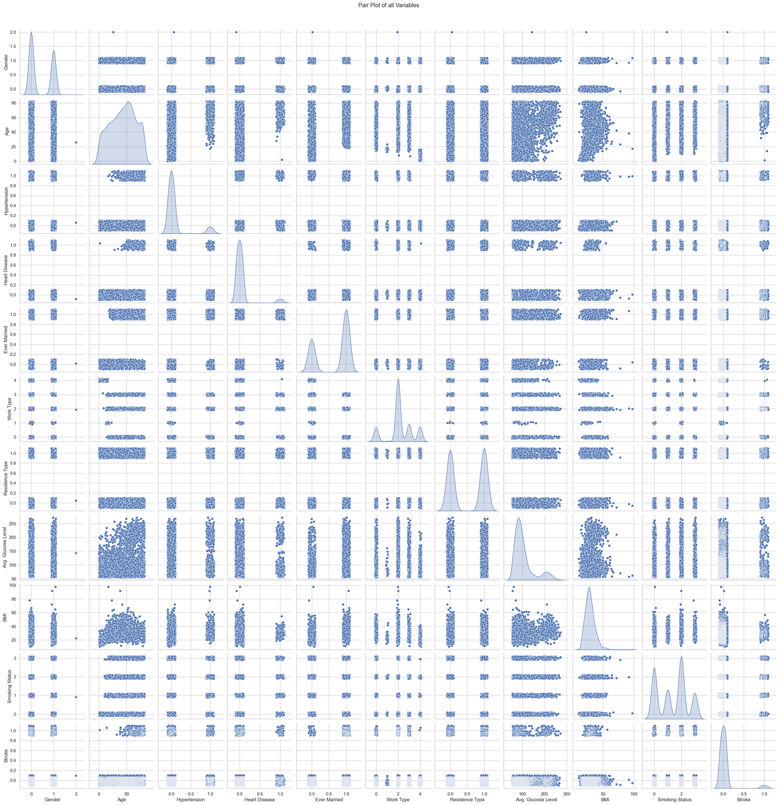
Pairplot of all variables with random noise
The graphs below show the result of the calculated correlation matrix for the entire dataset next to the correlation values of the variables in relation to the target variable stroke.
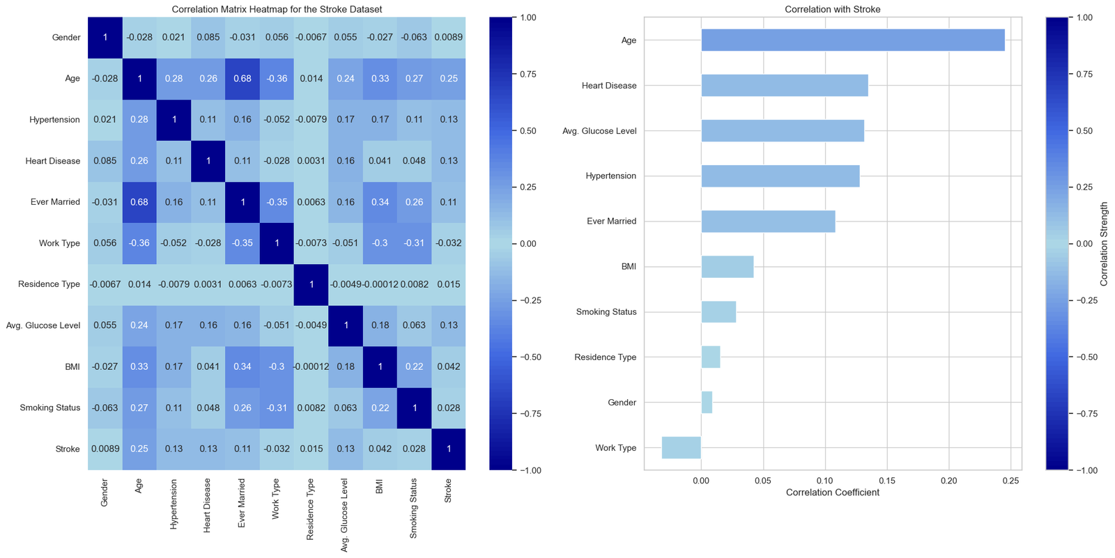
Correlation matrix and correlation coefficient for stroke as linear model
The correlation matrix shows Age, Heart Disease, Average Glucose Level and Hypertension as the main independent variables for stroke risk. Ever married shows a strong correlation with age, possibly indicating that marriage was more common in older generations. As such, Ever Married is likely to be a confounder in the context of stroke risk analysis.
Data Cleaning and Feature Engineering
To prepare the data for the further analysis and the modeling phase we will perform the following steps:
- Handling Missing Values: Address missing values as appropriate.
- Discretization - Handling of Outliers: Transforming continuos variables into categories for improved performance and explanation.
- Encoding Categorical Variables: Convert categorical variables into numerical format using one-hot encoding.
- Data Splitting: Split the data into training and testing sets.
- Feature Scaling: Scale features to ensure they are on a similar scale.
- Addressing unbalanced data: Balances the classes in the training set.
Handling Missing Values
The only variable showing missing values in the dataset id 'BMI'. There are 201 records with missing BMI value, from these 201 a count of 40 are stroke cases (Stroke =1). We will adjust the missing values by calculating the group mean BMI by gender, age and glocuse level.
Discretization - Handling of Outliers
By categorizing continuous variables into discrete groups, we can enhance the interpretability of the data and improve the performance of classification models by capturing non-linear relationships and reducing the influence of outliers.
For age, the dataset is divided into categories from 0-18 years, 18-30 years, 30-40 years, 40-50 years, 50-65 years, 65-75 years and more than 75 years. These categories reflect different life stages, which may correlate differently with stroke risk due to varying health behaviors and biological changes.
For BMI (Body Mass Index), the classification follows standard health guidelines: Underweight (BMI < 18.5), Normal Weight (18.5 ≤ BMI < 24.9), Overweight (25 ≤ BMI < 29.9), and Obese (BMI ≥ 30).
For glucose levels, categories are Normal (glucose < 140 mg/dL), Prediabetes (140 ≤ glucose < 200 mg/dL), and Diabetes (glucose ≥ 200 mg/dL).
The resulting distributions are shown below.

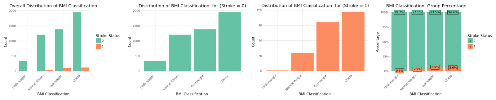
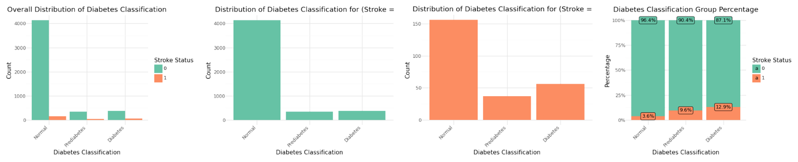
Distribution for grouped variables Age, BMI and Diabetes(Glucose Level)
Encoding categorical variables
To prepare the data for the modeling phase we will apply one hot encoding to all categorical variables. Two categorical variables are already encoded as numbers, these are 'hypertension' and 'heart_disease'. After performing the one hot encoding with omitting the default value (drop_first=true) the dataset is widened to 17 features including the target variable.
| count | mean | std | min | 25% | 50% | 75% | max | |
|---|---|---|---|---|---|---|---|---|
| hypertension | 5110.0 | 0.097456 | 0.296607 | 0.0 | 0.0 | 0.0 | 0.0 | 1.0 |
| heart_disease | 5110.0 | 0.054012 | 0.226063 | 0.0 | 0.0 | 0.0 | 0.0 | 1.0 |
| stroke | 5110.0 | 0.048728 | 0.215320 | 0.0 | 0.0 | 0.0 | 0.0 | 1.0 |
| glucose_group | 5110.0 | 0.245597 | 0.595996 | 0.0 | 0.0 | 0.0 | 0.0 | 2.0 |
| age_group | 5110.0 | 2.846184 | 1.915983 | 0.0 | 1.0 | 3.0 | 4.0 | 6.0 |
| bmi_group | 5110.0 | 2.028963 | 0.952761 | 0.0 | 1.0 | 2.0 | 3.0 | 3.0 |
| gender_Male | 5110.0 | 0.413894 | 0.492578 | 0.0 | 0.0 | 0.0 | 1.0 | 1.0 |
| gender_Other | 5110.0 | 0.000196 | 0.013989 | 0.0 | 0.0 | 0.0 | 0.0 | 1.0 |
| ever_married_Yes | 5110.0 | 0.656164 | 0.475034 | 0.0 | 0.0 | 1.0 | 1.0 | 1.0 |
| work_type_Never_worked | 5110.0 | 0.004305 | 0.065480 | 0.0 | 0.0 | 0.0 | 0.0 | 1.0 |
| work_type_Private | 5110.0 | 0.572407 | 0.494778 | 0.0 | 0.0 | 1.0 | 1.0 | 1.0 |
| work_type_Self-employed | 5110.0 | 0.160274 | 0.366896 | 0.0 | 0.0 | 0.0 | 0.0 | 1.0 |
| work_type_children | 5110.0 | 0.134442 | 0.341160 | 0.0 | 0.0 | 0.0 | 0.0 | 1.0 |
| Residence_type_Urban | 5110.0 | 0.508023 | 0.499985 | 0.0 | 0.0 | 1.0 | 1.0 | 1.0 |
| smoking_status_formerly smoked | 5110.0 | 0.173190 | 0.378448 | 0.0 | 0.0 | 0.0 | 0.0 | 1.0 |
| smoking_status_never smoked | 5110.0 | 0.370254 | 0.482920 | 0.0 | 0.0 | 0.0 | 1.0 | 1.0 |
| smoking_status_smokes | 5110.0 | 0.154403 | 0.361370 | 0.0 | 0.0 | 0.0 | 0.0 | 1.0 |
Data splitting
In the next step we split the data in a ratio of 70/30 into training and test sets, whilst maintaining the class distribution with stratify=y.
| Dataset | Shape | |
|---|---|---|
| 0 | Training Features | (3577, 16) |
| 1 | Test Features | (1533, 16) |
| 2 | Training Target | (3577,) |
| 3 | Test Target | (1533,) |
Feature Scaling
Scaling is crucial for ensuring that algorithms, which are sensitive to the scale of the input data, perform optimally and produce reliable results. We apply a MinMax scaler to the stroke data to normalize the features so that they have a value between 0 and 1.
| count | mean | std | min | 25% | 50% | 75% | max | |
|---|---|---|---|---|---|---|---|---|
| hypertension | 3577.0 | 0.096170 | 0.294865 | 0.0 | 0.000000 | 0.000000 | 0.000000 | 1.0 |
| heart_disease | 3577.0 | 0.053956 | 0.225962 | 0.0 | 0.000000 | 0.000000 | 0.000000 | 1.0 |
| glucose_group | 3577.0 | 0.120352 | 0.295112 | 0.0 | 0.000000 | 0.000000 | 0.000000 | 1.0 |
| age_group | 3577.0 | 0.474839 | 0.317024 | 0.0 | 0.166667 | 0.500000 | 0.666667 | 1.0 |
| bmi_group | 3577.0 | 0.675240 | 0.319805 | 0.0 | 0.333333 | 0.666667 | 1.000000 | 1.0 |
| gender_Male | 3577.0 | 0.414593 | 0.492721 | 0.0 | 0.000000 | 0.000000 | 1.000000 | 1.0 |
| gender_Other | 3577.0 | 0.000280 | 0.016720 | 0.0 | 0.000000 | 0.000000 | 0.000000 | 1.0 |
| ever_married_Yes | 3577.0 | 0.660050 | 0.473758 | 0.0 | 0.000000 | 1.000000 | 1.000000 | 1.0 |
| work_type_Never_worked | 3577.0 | 0.003355 | 0.057831 | 0.0 | 0.000000 | 0.000000 | 0.000000 | 1.0 |
| work_type_Private | 3577.0 | 0.571429 | 0.494941 | 0.0 | 0.000000 | 1.000000 | 1.000000 | 1.0 |
| work_type_Self-employed | 3577.0 | 0.164663 | 0.370928 | 0.0 | 0.000000 | 0.000000 | 0.000000 | 1.0 |
| work_type_children | 3577.0 | 0.134470 | 0.341205 | 0.0 | 0.000000 | 0.000000 | 0.000000 | 1.0 |
| Residence_type_Urban | 3577.0 | 0.504054 | 0.500053 | 0.0 | 0.000000 | 1.000000 | 1.000000 | 1.0 |
| smoking_status_formerly smoked | 3577.0 | 0.176405 | 0.381217 | 0.0 | 0.000000 | 0.000000 | 0.000000 | 1.0 |
| smoking_status_never smoked | 3577.0 | 0.370981 | 0.483135 | 0.0 | 0.000000 | 0.000000 | 1.000000 | 1.0 |
| smoking_status_smokes | 3577.0 | 0.149567 | 0.356696 | 0.0 | 0.000000 | 0.000000 | 0.000000 | 1.0 |
Addressing unbalanced dataset
The imbalance of the dataset can lead to biased models that are heavily skewed towards predicting the majority class, thereby compromising the model's ability to correctly identify and predict strokes. We will apply SMOTE (Synthetic Minority Over-sampling Technique) and alternatively Random Undersampling to the stroke dataset to address the significant class imbalance. This should enhance recall results, which is critical for developing predictive models in healthcare.
4. Model Training
During model training we will evaluate six classification models as listed below. To optimize these models, we will tune hyperparameters using GridSearchCV with a 5-fold cross-validation. This approach ensures that our models are robust and generalize well to unseen data. In addition to hyperparameter tuning, we will explore different resampling methods to address class imbalance, specifically using SMOTE (Synthetic Minority Over-sampling Technique) and random undersampling. To comprehensively evaluate model performance, we will vary the scoring metrics used in GridSearchCV, including F1 score, recall, and F-beta scores with beta values of 2 and 4. These varied scoring metrics will help us assess the models' ability to balance precision and recall, particularly emphasizing recall with the higher beta values in the F-beta score. This extensive evaluation process aims to identify the most effective model scoring and resampling strategy for predicting stroke risk.
Classification Models
The following classification models have been selected for the analysis.
- Logistic Regression with Regularization: Used as a baseline model for its simplicity and interpretability.
- KNN: A non-parametric method used for classification by comparing a test sample to the 'k' nearest neighbors in the feature space.
- Decision Tree: A model that uses a tree-like graph of decisions and their possible consequences, known for its simplicity and ability to handle non-linear relationships.
- Naive Bayes: A probabilistic classifier based on Bayes' theorem, assuming independence between predictors. It's particularly effective for problems with categorical input data.
- AdaBoost: An ensemble method that combines multiple weak classifiers to create a strong classifier. It works by iteratively training classifiers and adjusting their weights to focus on misclassified instances, improving overall model performance.
- Random Forest: Another ensemble method that constructs multiple decision trees during training and outputs the mode of the classes (classification) or the mean prediction (regression) of the individual trees. This method controls overfitting by averaging multiple decision trees, each built from a random subset of the training data and features.
Model Evaluation
The models where evaluated using the same training and test splits for all models to ensure fair comparison. The evaluation methods that were used to evaluate the models were:
Performance Indicators
- Accuracy
- Precision
- Recall
- F1 score as F1
- FBeta score for beta=2 as F2
- FBeta score for beta=4 as F4
Confusion Matrix
- True positive (1) and False positive (1) counts
- True negative (0) and False negative (0) counts
The results of these metrics for a total of 48 different combinations of resampling method, cross validation scoring and model are shown in the tables below sorted by the F4 score. In each combination the best hyperparameters for the model were determined before calculating the performance indicators.
Results - Performance Indicators
| Resampling | Scoring | Model | Precision | Recall | Accuracy | F1 | F2 | F4 | |
|---|---|---|---|---|---|---|---|---|---|
| 0 | SMOTE | f1 | Logistic Regression | 0.1096 | 0.8400 | 0.6582 | 0.1938 | 0.3600 | 0.6034 |
| 6 | SMOTE | recall | Logistic Regression | 0.1096 | 0.8400 | 0.6582 | 0.1938 | 0.3600 | 0.6034 |
| 12 | SMOTE | f2 | Logistic Regression | 0.1096 | 0.8400 | 0.6582 | 0.1938 | 0.3600 | 0.6034 |
| 18 | SMOTE | f4 | Logistic Regression | 0.1096 | 0.8400 | 0.6582 | 0.1938 | 0.3600 | 0.6034 |
| 16 | SMOTE | f2 | AdaBoost | 0.1009 | 0.8667 | 0.6158 | 0.1808 | 0.3443 | 0.5992 |
| 22 | SMOTE | f4 | AdaBoost | 0.0988 | 0.8667 | 0.6067 | 0.1774 | 0.3392 | 0.5947 |
| 38 | Undersampling | f2 | Decision Tree | 0.1204 | 0.7867 | 0.7084 | 0.2088 | 0.3734 | 0.5935 |
| 44 | Undersampling | f4 | Decision Tree | 0.1204 | 0.7867 | 0.7084 | 0.2088 | 0.3734 | 0.5935 |
| 32 | Undersampling | recall | Decision Tree | 0.1204 | 0.7867 | 0.7084 | 0.2088 | 0.3734 | 0.5935 |
| 26 | Undersampling | f1 | Decision Tree | 0.1204 | 0.7867 | 0.7084 | 0.2088 | 0.3734 | 0.5935 |
| 40 | Undersampling | f2 | AdaBoost | 0.0973 | 0.8667 | 0.6001 | 0.1750 | 0.3357 | 0.5915 |
| 42 | Undersampling | f4 | Logistic Regression | 0.0973 | 0.8667 | 0.6001 | 0.1750 | 0.3357 | 0.5915 |
| 34 | Undersampling | recall | AdaBoost | 0.0973 | 0.8667 | 0.6001 | 0.1750 | 0.3357 | 0.5915 |
| 30 | Undersampling | recall | Logistic Regression | 0.0973 | 0.8667 | 0.6001 | 0.1750 | 0.3357 | 0.5915 |
| 46 | Undersampling | f4 | AdaBoost | 0.0973 | 0.8667 | 0.6001 | 0.1750 | 0.3357 | 0.5915 |
| 28 | Undersampling | f1 | AdaBoost | 0.0973 | 0.8667 | 0.6001 | 0.1750 | 0.3357 | 0.5915 |
| 36 | Undersampling | f2 | Logistic Regression | 0.0973 | 0.8667 | 0.6001 | 0.1750 | 0.3357 | 0.5915 |
| 24 | Undersampling | f1 | Logistic Regression | 0.0973 | 0.8667 | 0.6001 | 0.1750 | 0.3357 | 0.5915 |
| 10 | SMOTE | recall | AdaBoost | 0.0973 | 0.8667 | 0.6001 | 0.1750 | 0.3357 | 0.5915 |
| 3 | SMOTE | f1 | Naive Bayes | 0.0808 | 0.9467 | 0.4703 | 0.1488 | 0.3011 | 0.5806 |
| 15 | SMOTE | f2 | Naive Bayes | 0.0723 | 0.9867 | 0.3803 | 0.1348 | 0.2797 | 0.5659 |
| 39 | Undersampling | f2 | Naive Bayes | 0.0711 | 0.9867 | 0.3686 | 0.1326 | 0.2759 | 0.5614 |
| 27 | Undersampling | f1 | Naive Bayes | 0.0841 | 0.8667 | 0.5316 | 0.1533 | 0.3029 | 0.5601 |
| 47 | Undersampling | f4 | Random Forest | 0.1071 | 0.7600 | 0.6784 | 0.1878 | 0.3425 | 0.5595 |
| 41 | Undersampling | f2 | Random Forest | 0.1071 | 0.7600 | 0.6784 | 0.1878 | 0.3425 | 0.5595 |
| 29 | Undersampling | f1 | Random Forest | 0.1071 | 0.7600 | 0.6784 | 0.1878 | 0.3425 | 0.5595 |
| 43 | Undersampling | f4 | K-Nearest Neighbors | 0.0988 | 0.7867 | 0.6386 | 0.1756 | 0.3289 | 0.5582 |
| 25 | Undersampling | f1 | K-Nearest Neighbors | 0.0988 | 0.7867 | 0.6386 | 0.1756 | 0.3289 | 0.5582 |
| 31 | Undersampling | recall | K-Nearest Neighbors | 0.0988 | 0.7867 | 0.6386 | 0.1756 | 0.3289 | 0.5582 |
| 37 | Undersampling | f2 | K-Nearest Neighbors | 0.0988 | 0.7867 | 0.6386 | 0.1756 | 0.3289 | 0.5582 |
| 35 | Undersampling | recall | Random Forest | 0.1059 | 0.7600 | 0.6745 | 0.1860 | 0.3401 | 0.5575 |
| 21 | SMOTE | f4 | Naive Bayes | 0.0672 | 0.9867 | 0.3294 | 0.1259 | 0.2641 | 0.5467 |
| 45 | Undersampling | f4 | Naive Bayes | 0.0661 | 0.9867 | 0.3170 | 0.1238 | 0.2606 | 0.5422 |
| 4 | SMOTE | f1 | AdaBoost | 0.0966 | 0.7600 | 0.6406 | 0.1714 | 0.3202 | 0.5413 |
| 33 | Undersampling | recall | Naive Bayes | 0.0651 | 0.9867 | 0.3059 | 0.1221 | 0.2575 | 0.5383 |
| 9 | SMOTE | recall | Naive Bayes | 0.0562 | 0.9867 | 0.1885 | 0.1063 | 0.2288 | 0.4998 |
| 19 | SMOTE | f4 | K-Nearest Neighbors | 0.0911 | 0.4667 | 0.7462 | 0.1525 | 0.2558 | 0.3756 |
| 7 | SMOTE | recall | K-Nearest Neighbors | 0.0911 | 0.4667 | 0.7462 | 0.1525 | 0.2558 | 0.3756 |
| 13 | SMOTE | f2 | K-Nearest Neighbors | 0.0911 | 0.4667 | 0.7462 | 0.1525 | 0.2558 | 0.3756 |
| 1 | SMOTE | f1 | K-Nearest Neighbors | 0.0985 | 0.4400 | 0.7756 | 0.1610 | 0.2598 | 0.3655 |
| 8 | SMOTE | recall | Decision Tree | 0.0930 | 0.2667 | 0.8369 | 0.1379 | 0.1942 | 0.2403 |
| 14 | SMOTE | f2 | Decision Tree | 0.0930 | 0.2667 | 0.8369 | 0.1379 | 0.1942 | 0.2403 |
| 20 | SMOTE | f4 | Decision Tree | 0.0930 | 0.2667 | 0.8369 | 0.1379 | 0.1942 | 0.2403 |
| 2 | SMOTE | f1 | Decision Tree | 0.0930 | 0.2667 | 0.8369 | 0.1379 | 0.1942 | 0.2403 |
| 11 | SMOTE | recall | Random Forest | 0.0941 | 0.2533 | 0.8441 | 0.1372 | 0.1892 | 0.2304 |
| 23 | SMOTE | f4 | Random Forest | 0.0941 | 0.2533 | 0.8441 | 0.1372 | 0.1892 | 0.2304 |
| 17 | SMOTE | f2 | Random Forest | 0.0838 | 0.2133 | 0.8474 | 0.1203 | 0.1629 | 0.1955 |
| 5 | SMOTE | f1 | Random Forest | 0.0789 | 0.2000 | 0.8467 | 0.1132 | 0.1531 | 0.1835 |
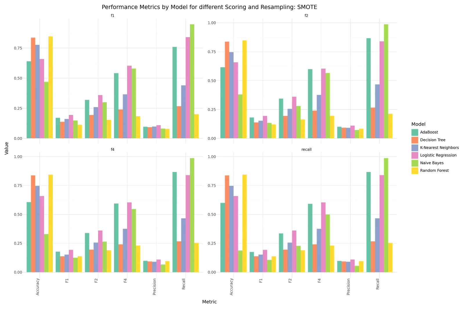
Performance Results for SMOTE resampling and different cross validation scoring
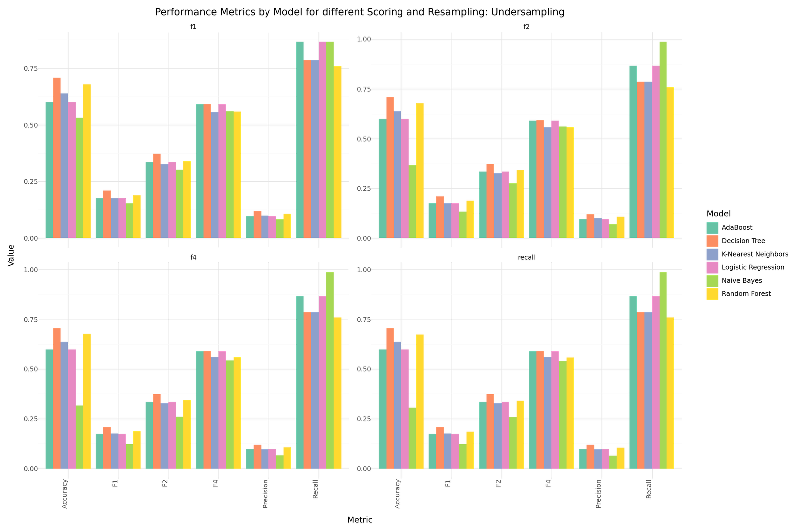
Performance Results for Random Undersampling resampling and different cross validation scoring
The models were optimized with different scoring criteria to focus on recall and a weighted fbeta score in favor of avoiding misclassification of true stroke risk patients. The results in the tables are sorted by the F4 score as fbeta with beta=4. THe results show the best performance for Logistic regression models trained with SMOTE sampled data, followed by two AdaBoost model also trained with SMOTE sampled data before four Decision Tree models trained with Random Undersampled data. Regading the resampling method it can be observed that DecisionTrees, RandomForest and KNN models perform better when trained with Random Undersampled data. In contrast Logistic Regression, Naive Bayes and AdaBoost show better results when they are trained applying Oversampling with SMOTE.
Results - Confusion Matrix
| Resampling | Scoring | Model | F4 | True 1 | True 0 | False 1 | False 0 | |
|---|---|---|---|---|---|---|---|---|
| 0 | SMOTE | f1 | Logistic Regression | 0.6034 | 63 | 946 | 512 | 12 |
| 6 | SMOTE | recall | Logistic Regression | 0.6034 | 63 | 946 | 512 | 12 |
| 12 | SMOTE | f2 | Logistic Regression | 0.6034 | 63 | 946 | 512 | 12 |
| 18 | SMOTE | f4 | Logistic Regression | 0.6034 | 63 | 946 | 512 | 12 |
| 16 | SMOTE | f2 | AdaBoost | 0.5992 | 65 | 879 | 579 | 10 |
| 22 | SMOTE | f4 | AdaBoost | 0.5947 | 65 | 865 | 593 | 10 |
| 38 | Undersampling | f2 | Decision Tree | 0.5935 | 59 | 1027 | 431 | 16 |
| 44 | Undersampling | f4 | Decision Tree | 0.5935 | 59 | 1027 | 431 | 16 |
| 32 | Undersampling | recall | Decision Tree | 0.5935 | 59 | 1027 | 431 | 16 |
| 26 | Undersampling | f1 | Decision Tree | 0.5935 | 59 | 1027 | 431 | 16 |
| 40 | Undersampling | f2 | AdaBoost | 0.5915 | 65 | 855 | 603 | 10 |
| 42 | Undersampling | f4 | Logistic Regression | 0.5915 | 65 | 855 | 603 | 10 |
| 34 | Undersampling | recall | AdaBoost | 0.5915 | 65 | 855 | 603 | 10 |
| 30 | Undersampling | recall | Logistic Regression | 0.5915 | 65 | 855 | 603 | 10 |
| 46 | Undersampling | f4 | AdaBoost | 0.5915 | 65 | 855 | 603 | 10 |
| 28 | Undersampling | f1 | AdaBoost | 0.5915 | 65 | 855 | 603 | 10 |
| 36 | Undersampling | f2 | Logistic Regression | 0.5915 | 65 | 855 | 603 | 10 |
| 24 | Undersampling | f1 | Logistic Regression | 0.5915 | 65 | 855 | 603 | 10 |
| 10 | SMOTE | recall | AdaBoost | 0.5915 | 65 | 855 | 603 | 10 |
| 3 | SMOTE | f1 | Naive Bayes | 0.5806 | 71 | 650 | 808 | 4 |
| 15 | SMOTE | f2 | Naive Bayes | 0.5659 | 74 | 509 | 949 | 1 |
| 39 | Undersampling | f2 | Naive Bayes | 0.5614 | 74 | 491 | 967 | 1 |
| 27 | Undersampling | f1 | Naive Bayes | 0.5601 | 65 | 750 | 708 | 10 |
| 47 | Undersampling | f4 | Random Forest | 0.5595 | 57 | 983 | 475 | 18 |
| 41 | Undersampling | f2 | Random Forest | 0.5595 | 57 | 983 | 475 | 18 |
| 29 | Undersampling | f1 | Random Forest | 0.5595 | 57 | 983 | 475 | 18 |
| 43 | Undersampling | f4 | K-Nearest Neighbors | 0.5582 | 59 | 920 | 538 | 16 |
| 25 | Undersampling | f1 | K-Nearest Neighbors | 0.5582 | 59 | 920 | 538 | 16 |
| 31 | Undersampling | recall | K-Nearest Neighbors | 0.5582 | 59 | 920 | 538 | 16 |
| 37 | Undersampling | f2 | K-Nearest Neighbors | 0.5582 | 59 | 920 | 538 | 16 |
| 35 | Undersampling | recall | Random Forest | 0.5575 | 57 | 977 | 481 | 18 |
| 21 | SMOTE | f4 | Naive Bayes | 0.5467 | 74 | 431 | 1027 | 1 |
| 45 | Undersampling | f4 | Naive Bayes | 0.5422 | 74 | 412 | 1046 | 1 |
| 4 | SMOTE | f1 | AdaBoost | 0.5413 | 57 | 925 | 533 | 18 |
| 33 | Undersampling | recall | Naive Bayes | 0.5383 | 74 | 395 | 1063 | 1 |
| 9 | SMOTE | recall | Naive Bayes | 0.4998 | 74 | 215 | 1243 | 1 |
| 19 | SMOTE | f4 | K-Nearest Neighbors | 0.3756 | 35 | 1109 | 349 | 40 |
| 7 | SMOTE | recall | K-Nearest Neighbors | 0.3756 | 35 | 1109 | 349 | 40 |
| 13 | SMOTE | f2 | K-Nearest Neighbors | 0.3756 | 35 | 1109 | 349 | 40 |
| 1 | SMOTE | f1 | K-Nearest Neighbors | 0.3655 | 33 | 1156 | 302 | 42 |
| 8 | SMOTE | recall | Decision Tree | 0.2403 | 20 | 1263 | 195 | 55 |
| 14 | SMOTE | f2 | Decision Tree | 0.2403 | 20 | 1263 | 195 | 55 |
| 20 | SMOTE | f4 | Decision Tree | 0.2403 | 20 | 1263 | 195 | 55 |
| 2 | SMOTE | f1 | Decision Tree | 0.2403 | 20 | 1263 | 195 | 55 |
| 11 | SMOTE | recall | Random Forest | 0.2304 | 19 | 1275 | 183 | 56 |
| 23 | SMOTE | f4 | Random Forest | 0.2304 | 19 | 1275 | 183 | 56 |
| 17 | SMOTE | f2 | Random Forest | 0.1955 | 16 | 1283 | 175 | 59 |
| 5 | SMOTE | f1 | Random Forest | 0.1835 | 15 | 1283 | 175 | 60 |
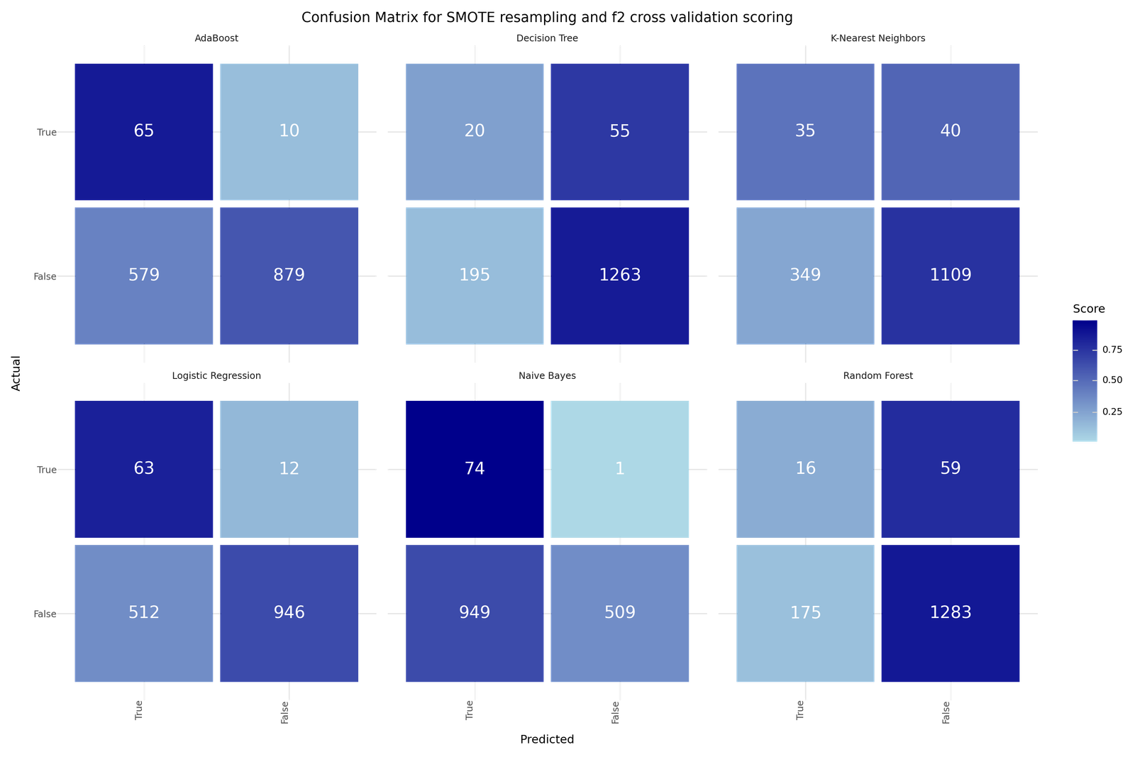
Confusion Matrices for SMOTE and f2 cross validation scoring
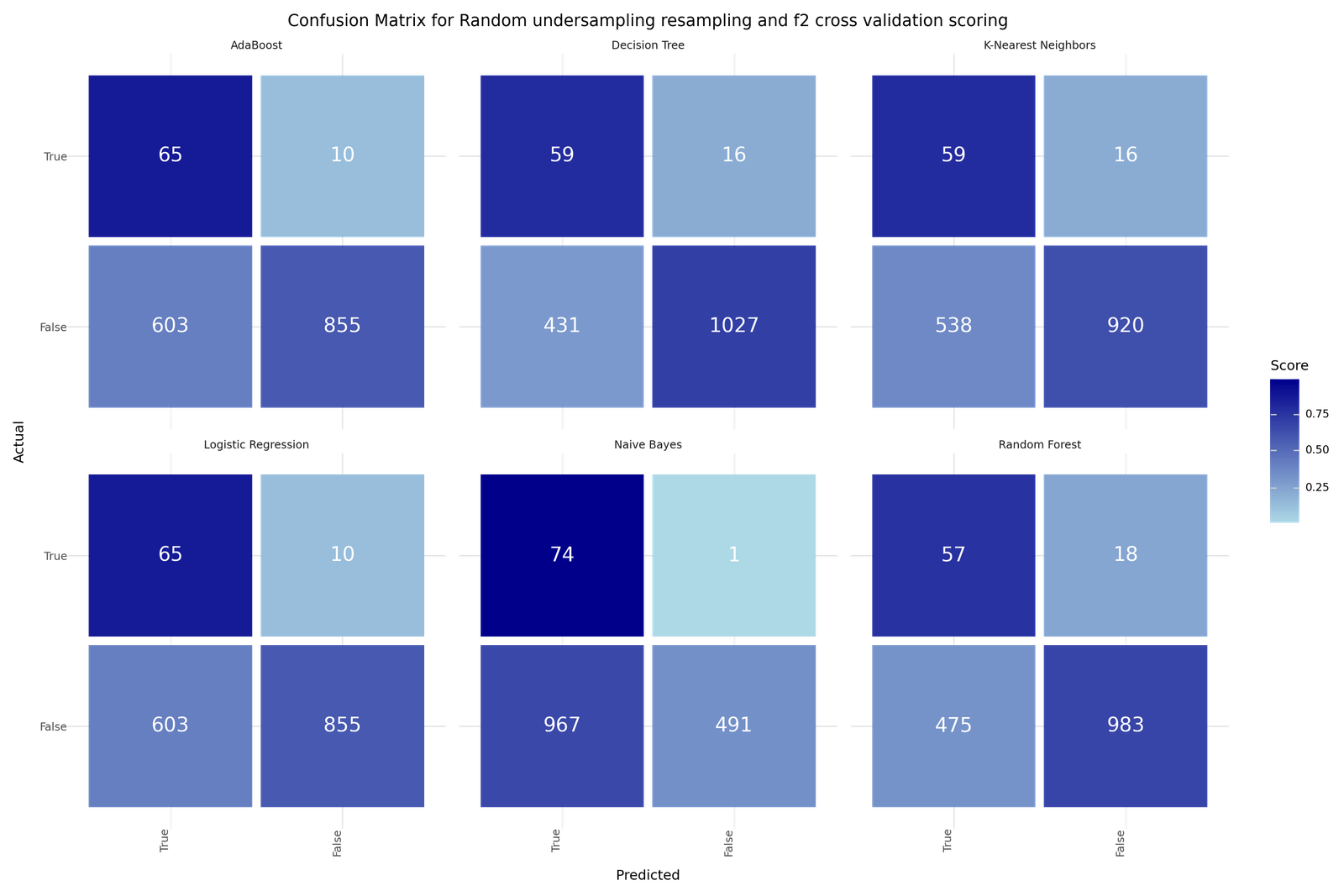
Confusion Matrices for Random Undersampling and f2 cross validation scoring
If we would aim purely to minimize the Type II error, meaning trying to avoid misclassifying true stroke risk cases, we would find the smallest Type II error counts in the Naive Bayes models. Model 15 as an example misclassifies only one true stroke case of the test dataset falsely as stroke=0. Unfortunately the good performance at finding true stroke cases comes at the cost of big counts of Type I errors, non stroke patients that were identified as stroke risk patients. Naive Bayes model 15 produced 949 Type I errors out of 1458 non stroke cases. The Logistic Regression models deliver a more balanced result. The best out of the 8 Logistic Regression Models, Model 0, produced 12 Type II errors out of 75 stroke cases in the test data and 512 Type I errors out of 1458 non stroke cases. Also AdaBoost and Decision Tree models show good balance in terms of Type II vs Type I error counts. AdaBoost Model 16, produced 10 Type II errors out of 75 stroke cases in the test data and 579 Type I errors out of 1458 non stroke cases. Decision Tree Model 38, produced 16 Type II errors out of 75 stroke cases in the test data but only 431 Type I errors out of 1458 non stroke cases.
Results - Influence of features
To understand how the different algorithms used the values of different features to build a classification model, we select the best performing model for each of the algorithm and extract the available information about the feature influences. The results are shown in the bargraphs above the model specific confusion matrices below.
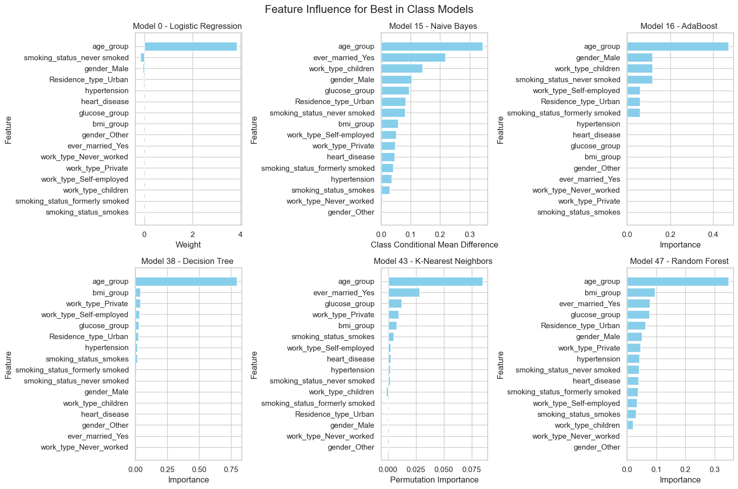
Feature Influence for Best in Class Models
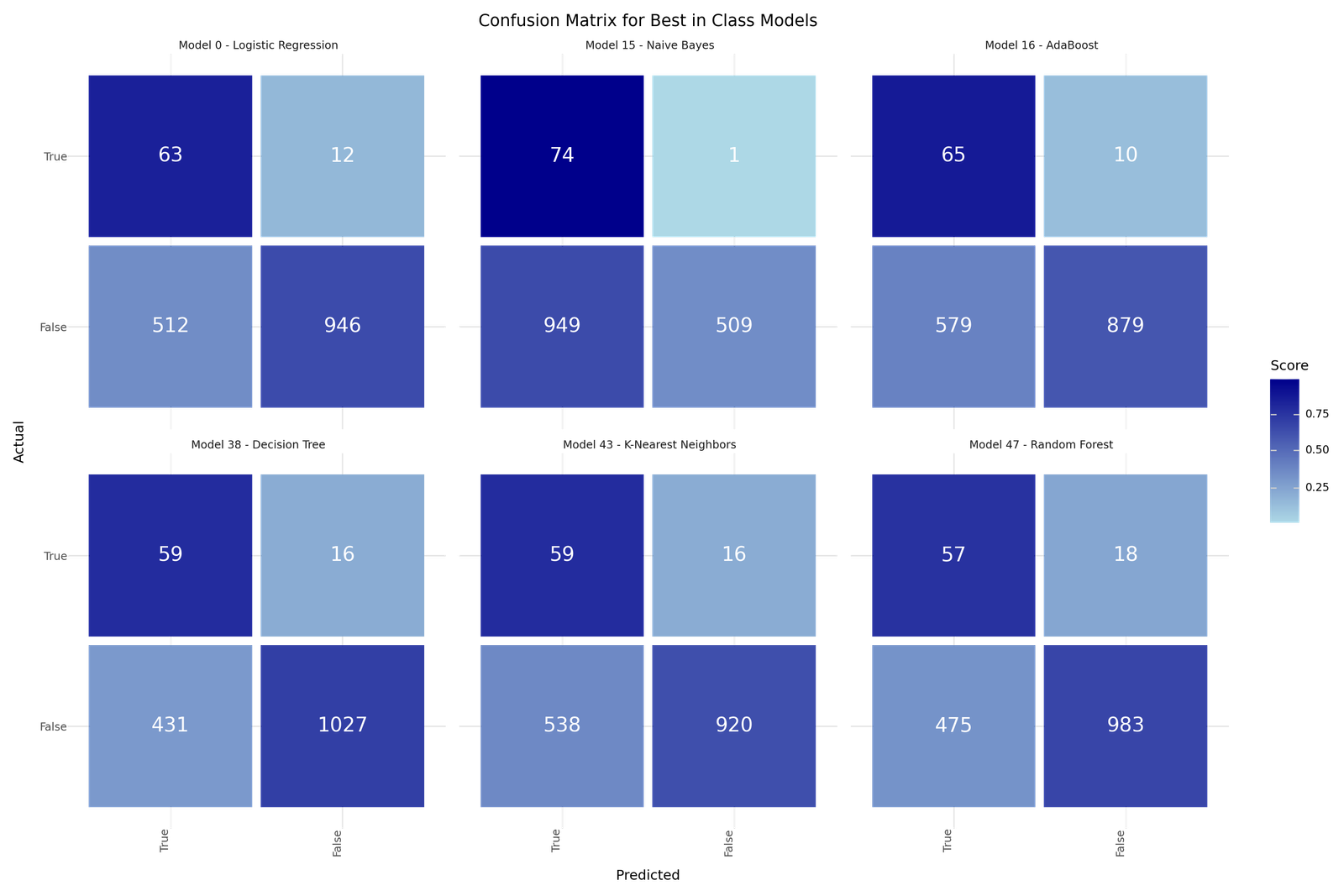
Confusion Matrix for Best in Class Models
We can see that age is the predominant influencing feature for all models. The Logistic Regression Model 0 uses L1 Regularization and eliminates most of the other features. The Random Forest and Naive Bayes classifier models show a wider use of features for their classification and allow better explanation than just age. From the exploratory analysis we would have summarized that age is most crucial but also BMI, Diabetes condition and heart disease have some influence on the stroke risk distribution. The feature extraction doesn't show otherwise but mainly confirm the influence of age.
5. Recommended Models
After training and evaluating the models, it is hard to identify a single best model. We would vote for Model 16 AdaBoost as best overall model as it has a low Type II error count but also a decent Type I error performance. As benchmark we would define an ensemble of models and predict based on the majority of "votes" of the models. For the ensemble we include the following models for best results in terms of:
-
Best overall: Model 16 - AdaBoost
-
Precision: Model 38 - Decision Tree
-
Type I error: Model 17 - Random Forest
-
Type II error: Model 15 - Naive Bayes
-
F4 score: Model 0 - Logistic Regression with L1 Regularization
-
F1 score: Model 41 - Random Forest
Best Model - Overall
The AdaBoost Model 16 shows a low Type II error count but also a decent Type I error performance, good accuracy and robust performance across different metrics.
[H]
10 1.2| Model 16 - AdaBoost | |
|---|---|
| Resampling | SMOTE |
| Scoring | f2 |
| Model | AdaBoost |
| Precision | 0.100932 |
| Recall | 0.866667 |
| Accuracy | 0.615786 |
| F1 | 0.180807 |
| F2 | 0.34428 |
| F4 | 0.599241 |
| True 1 | 65 |
| True 0 | 879 |
| False 1 | 579 |
| False 0 | 10 |
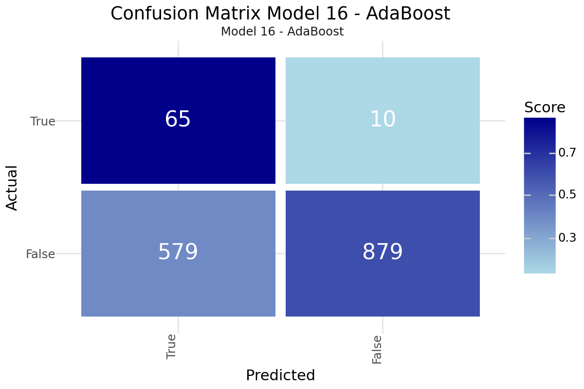

Confusion Matrix and Feature Influence for AdaBoost Model 16
Best Model - Precision
The Decision Tree Model 38 provides the highest Precision score, good accuracy and robust performance across different metrics.
[H]
10 1.2| Model 38 - Decision Tree | |
|---|---|
| Resampling | Undersampling |
| Scoring | f2 |
| Model | Decision Tree |
| Precision | 0.120408 |
| Recall | 0.786667 |
| Accuracy | 0.708415 |
| F1 | 0.20885 |
| F2 | 0.373418 |
| F4 | 0.593491 |
| True 1 | 59 |
| True 0 | 1027 |
| False 1 | 431 |
| False 0 | 16 |
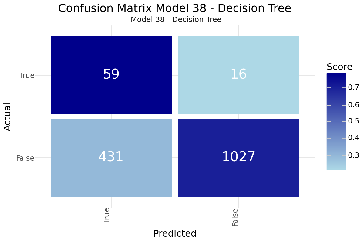
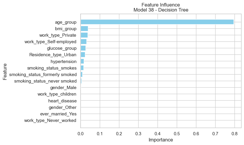
Confusion Matrix and Feature Influence for Decision Tree Model 38
Best Model - Type I error
The Random Forest Model 17 shows the lowest Type I error count, good explainability and good accuracy.
[H]
10 1.2| Model 17 - Random Forest | |
|---|---|
| Resampling | SMOTE |
| Scoring | f2 |
| Model | Random Forest |
| Precision | 0.08377 |
| Recall | 0.213333 |
| Accuracy | 0.847358 |
| F1 | 0.120301 |
| F2 | 0.162933 |
| F4 | 0.195543 |
| True 1 | 16 |
| True 0 | 1283 |
| False 1 | 175 |
| False 0 | 59 |
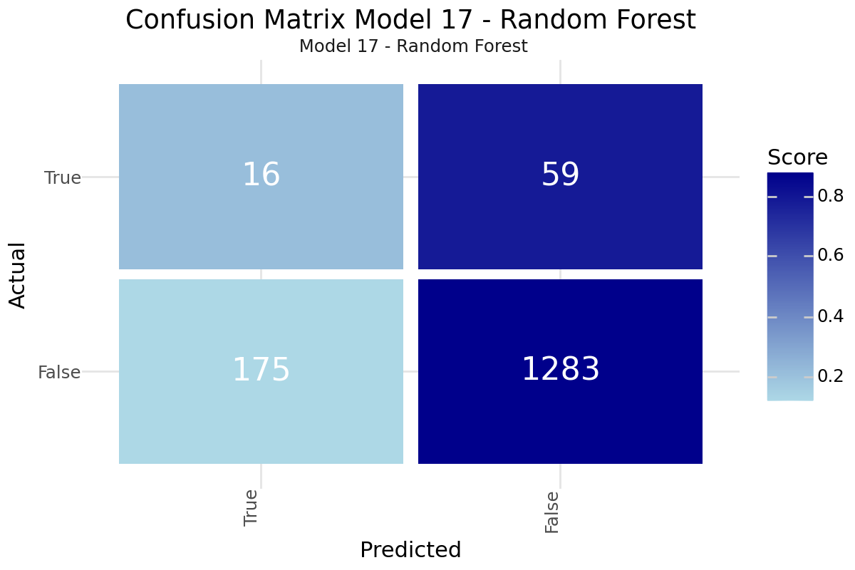
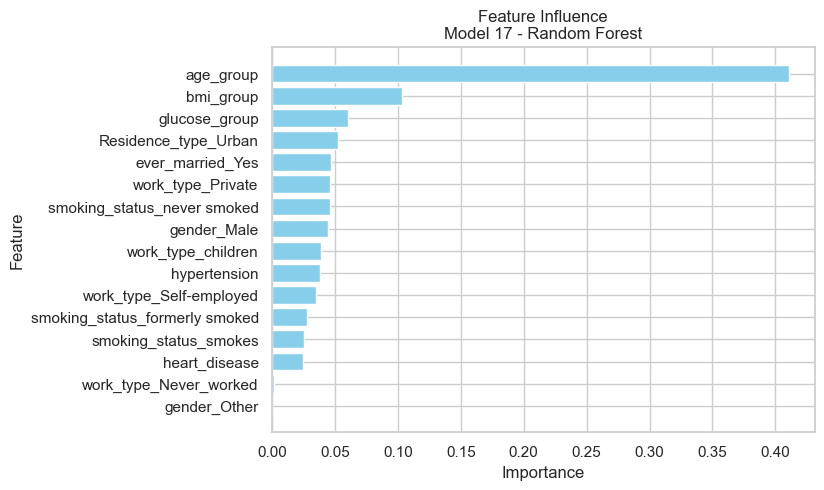
Confusion Matrix and Feature Influence for Random Forest Model 17
Best Model - Type II error
We were evaluating Naive Bayes Model 15 classifier achieves the best recall performance which should be helpful in avoiding too many Type II errors.
[H]
10 1.2| Model 15 - Naive Bayes | |
|---|---|
| Resampling | SMOTE |
| Scoring | f2 |
| Model | Naive Bayes |
| Precision | 0.072336 |
| Recall | 0.986667 |
| Accuracy | 0.3803 |
| F1 | 0.134791 |
| F2 | 0.279667 |
| F4 | 0.565902 |
| True 1 | 74 |
| True 0 | 509 |
| False 1 | 949 |
| False 0 | 1 |
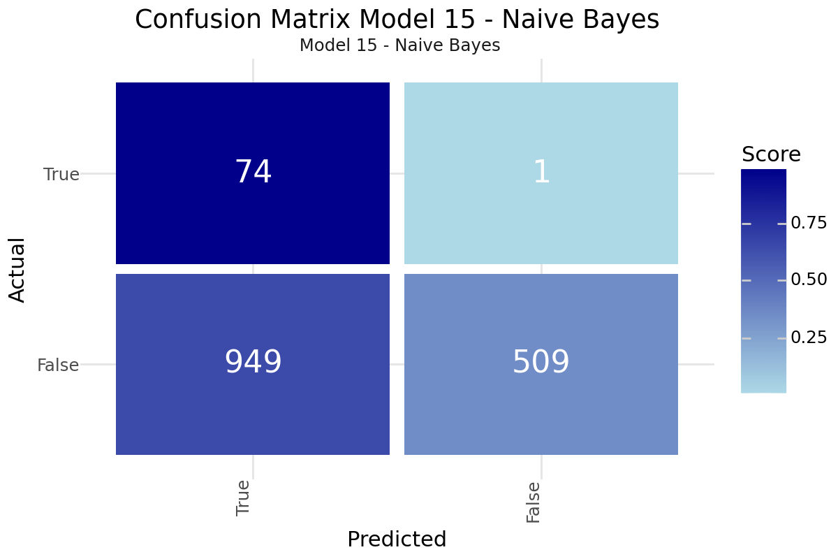

Confusion Matrix and Feature Influence for Naive Bayes Model 15
Best Model - F4 Score
The Logistic Regression Model 0 with L1 regularization provides the highest F4 score, good accuracy and robust performance across different metrics.
| Model 0 - Logistic Regression | |
|---|---|
| Resampling | SMOTE |
| Scoring | f1 |
| Model | Logistic Regression |
| Precision | 0.109565 |
| Recall | 0.84 |
| Accuracy | 0.658187 |
| F1 | 0.193846 |
| F2 | 0.36 |
| F4 | 0.60338 |
| True 1 | 63 |
| True 0 | 946 |
| False 1 | 512 |
| False 0 | 12 |
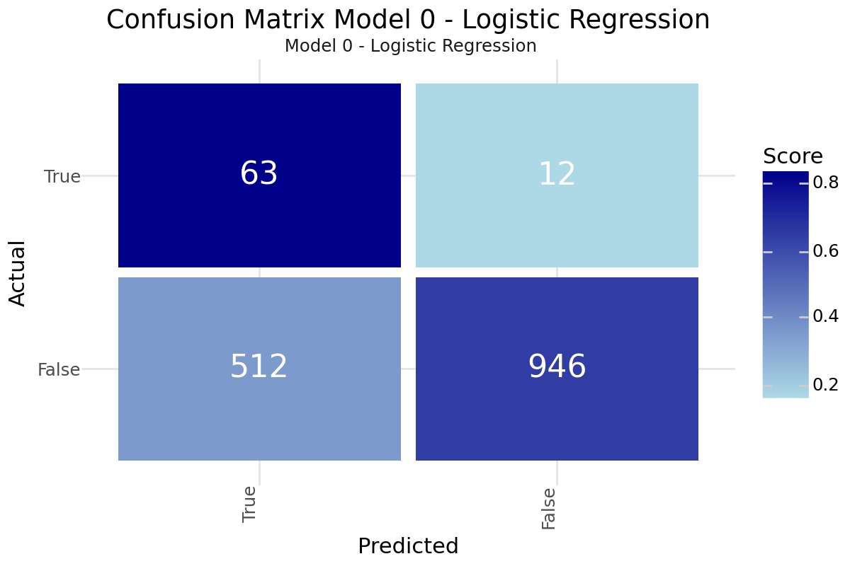
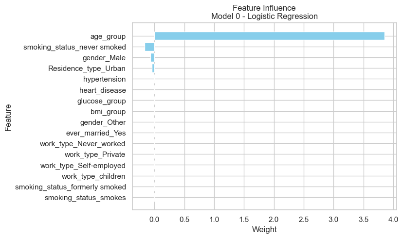
Confusion Matrix and Feature Influence for Logistic Regression Model 0
Best Model - F1 score
The Random Forest Model 41 offers the best F1 score after the Decision Tree and Logistic Regression Models that have already been selected. It shows good interpretability through the feature importance, making it easier to understand the key drivers of stroke risk.
[H]
10 1.2| Model 41 - Random Forest | |
|---|---|
| Resampling | Undersampling |
| Scoring | f2 |
| Model | Random Forest |
| Precision | 0.107143 |
| Recall | 0.76 |
| Accuracy | 0.678408 |
| F1 | 0.187809 |
| F2 | 0.342548 |
| F4 | 0.559469 |
| True 1 | 57 |
| True 0 | 983 |
| False 1 | 475 |
| False 0 | 18 |

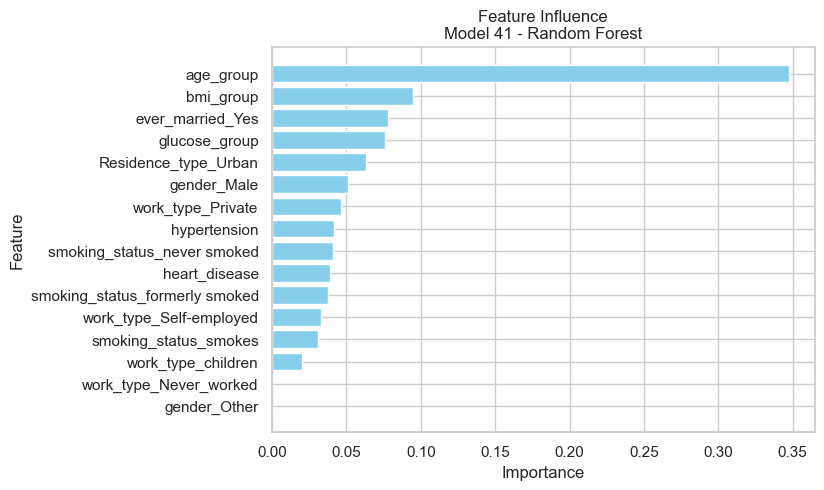
Confusion Matrix and Feature Influence for Random Forest Model 41
Ensemble Voting
All six models were used for an ensemble voting with the decision was made in favor of stroke risk for equal votes. The results show a very minor improvement compared to the overall best AdaBoost Model 16.
| ID | Model | Precision | Recall | Accuracy | F1 | F2 | F4 | |
|---|---|---|---|---|---|---|---|---|
| 0 | Model 16 | AdaBoost | 0.101 | 0.867 | 0.616 | 0.181 | 0.344 | 0.599 |
| 1 | Model 0 | Logistic Regression | 0.110 | 0.840 | 0.658 | 0.194 | 0.360 | 0.603 |
| 2 | Model 15 | Naive Bayes | 0.072 | 0.987 | 0.380 | 0.135 | 0.280 | 0.566 |
| 3 | Model 38 | Decision Tree | 0.120 | 0.787 | 0.708 | 0.209 | 0.373 | 0.593 |
| 4 | Model 17 | Random Forest | 0.084 | 0.213 | 0.847 | 0.120 | 0.163 | 0.196 |
| 5 | Model 41 | Random Forest | 0.107 | 0.760 | 0.678 | 0.188 | 0.343 | 0.559 |
| 6 | Model E | Ensemble | 0.101 | 0.867 | 0.616 | 0.181 | 0.345 | 0.600 |
| ID | Model | F4 | True 1 | True 0 | False 1 | False 0 | |
|---|---|---|---|---|---|---|---|
| 0 | Model 16 | AdaBoost | 0.599 | 65 | 879 | 579 | 10 |
| 1 | Model 0 | Logistic Regression | 0.603 | 63 | 946 | 512 | 12 |
| 2 | Model 15 | Naive Bayes | 0.566 | 74 | 509 | 949 | 1 |
| 3 | Model 38 | Decision Tree | 0.593 | 59 | 1027 | 431 | 16 |
| 4 | Model 17 | Random Forest | 0.196 | 16 | 1283 | 175 | 59 |
| 5 | Model 41 | Random Forest | 0.559 | 57 | 983 | 475 | 18 |
| 6 | Model E | Ensemble | 0.600 | 65 | 880 | 578 | 10 |
6. Key Findings and Insights
The analysis of the stroke prediction model has revealed several critical factors that significantly influence the likelihood of stroke in patients. Understanding these drivers allows for better-targeted interventions and more effective prevention strategies. However, to further enhance the accuracy and reliability of the model, additional data and features are essential.
Main Drivers influencing Stroke Risk
-
Age: Older patients have a higher risk of stroke. This finding underscores the importance of age-related health monitoring and interventions, as the likelihood of experiencing a stroke increases with age, necessitating enhanced medical vigilance for the elderly.
-
Hypertension: Presence of hypertension increases stroke risk. Hypertension, or high blood pressure, is a well-established risk factor for stroke, emphasizing the need for strict blood pressure control through medication, lifestyle changes, and regular monitoring.
-
Heart Disease: Patients with heart disease are more likely to experience a stroke. The strong correlation between cardiovascular conditions and stroke highlights the necessity for comprehensive care plans that address both heart disease management and stroke prevention.
-
Average Glucose Level: Higher average glucose levels are associated with Diabetes and increase stroke risk. Elevated glucose levels indicate poor diabetes control, which can lead to vascular damage and increased stroke risk, highlighting the importance of maintaining optimal glucose levels through diet, exercise, and medication adherence.
Insights
-
Preventive Measures: Targeted interventions for patients with hypertension and heart disease could reduce stroke incidence. Implementing comprehensive care plans that include lifestyle modifications, medication adherence, and regular health check-ups is crucial for mitigating stroke risk in these high-risk populations.
-
Public Health Strategies: Programs aimed at managing blood glucose levels and promoting healthy aging could be beneficial. Public health initiatives should focus on widespread screening for diabetes and hypertension, coupled with campaigns that encourage physical activity, healthy eating, and smoking cessation to reduce stroke risk at a population level.
-
Holistic Health Approach: Adopting a holistic approach that considers the interplay between various risk factors can enhance stroke prevention efforts. By addressing lifestyle factors such as diet, exercise, and stress management, healthcare providers can simultaneously mitigate risks associated with hypertension, heart disease, and diabetes, leading to better overall health outcomes.
-
Technology and Monitoring: Leveraging technology, such as wearable devices and telemedicine, can aid in the continuous monitoring of at-risk individuals. These technologies provide real-time data on blood pressure, glucose levels, and heart rate, allowing for timely interventions and personalized care plans that can significantly reduce stroke risk.
-
Education and Awareness: Raising awareness about the risk factors and preventive measures for stroke is crucial. Public health campaigns and educational programs should aim to inform individuals about the importance of regular health screenings, recognizing early symptoms of stroke, and seeking immediate medical attention, empowering them to take proactive steps towards stroke prevention.
Future Directions
To further improve the understanding and prediction of stroke risk, it is imperative to gather more comprehensive data and incorporate additional features into the model. Including a wider range of demographic, genetic, and lifestyle factors can provide a more nuanced view of stroke risk. Additionally, longitudinal data tracking patients over time could offer insights into how risk factors evolve and interact. By expanding the dataset and refining the features used, we can develop more accurate and robust models that enhance our ability to prevent and manage stroke.
7. Suggestions for Next Steps
-
Feature Enhancement: Incorporate additional health-related features, such as cholesterol levels, physical activity, and diet, to improve the model's predictive performance. Including more comprehensive lifestyle and biometric data can help create a more accurate and holistic risk assessment for stroke.
-
Longitudinal Data: Utilize longitudinal data to track changes in patient health over time, which can provide deeper insights into the progression and interaction of risk factors. Longitudinal studies allow for the observation of how individual risk profiles evolve, leading to more precise and personalized predictions.
-
Assessment of Existing Studies and Scores: Evaluate and integrate findings from established studies and scoring systems, such as the Framingham Heart Study and the CHA₂DS₂-VASc score, which are widely used for predicting cardiovascular and stroke risk. Comparing our model's performance with these well-regarded benchmarks can provide validation and highlight areas for improvement. Additionally, exploring datasets from these studies can offer valuable insights and potential features to enhance our model.
-
Collaborative Research: Engage in collaborative research with other institutions and researchers to leverage a broader range of expertise and datasets. By pooling resources and knowledge, we can develop more robust and generalizable models that are applicable across diverse populations.
-
Validation Across Diverse Populations: Test and validate the model across different demographic and geographic populations to ensure its applicability and reliability. Understanding how the model performs in various contexts can help identify any biases or limitations, leading to more equitable and effective stroke risk prediction tools.
-
Model Re-evaluation: Regularly update and re-evaluate the model as new data becomes available to ensure its continued relevance and accuracy. Incorporating the latest research findings and medical advancements will help maintain the model's effectiveness in predicting stroke risk.