Fresh and Rotten Fruits - Product inspection with Convolutional Neural Networks
The objective of this analysis is to develop a deep learning model that can accurately classify images of fresh and rotten fruits. We explored three models: a baseline Convolutional Neural Network (CNN), an enhanced CNN with Batch Normalization, and a VGG16-based model with pretrained layers. The analysis aims to automate fruit quality assessment, which is traditionally done manually and is both labor-intensive and error-prone. Automation is expected to reduce costs and improve efficiency for stakeholders like fruit distributors and retailers. The study utilized a diverse and realistic dataset, including augmented images, to ensure robust performance across various real-world conditions. Among the models tested, the CNN with Batch Normalization using Augmented Data achieved the highest validation accuracy of 95 Percent, making it the best-performing model in this study. This model not only provided the best accuracy but also balanced precision and recall, making it the most reliable for distinguishing between fresh and rotten fruits. The model's success demonstrates the effectiveness of augmentation and Batch Normalization in improving model performance while maintaining computational efficiency, making it well-suited for deployment in real-world fruit quality assessment tasks.
1. Objective of the Analysis
The primary goal of this analysis is to develop a robust deep learning model that can accurately classify images of fresh and rotten fruits. We will utilize a Convolutional Neural Network (CNN) due to its proven effectiveness in image classification tasks as base model. We will then extend the base model by Batch Normalization layers as a second model. As third model we include a pretrained model VGG16 with pretrained layers extented by customized final layers. This analysis is intended to assist stakeholders, including fruit distributors and retailers, by automating the process of assessing fruit quality. This automation can significantly reduce labor costs and minimize the errors associated with manual inspections.
Value of the Analysis
- Current Challenges: Typically, the task of distinguishing fresh from rotten fruits is performed manually, which is not only inefficient but also costly for fruit farmers and vendors. Therefore, creating an automated classification model is essential to reduce human effort, lower costs, and expedite production in the agriculture industry.
- Comprehensive Scope: Compared to other datasets, this one includes a wider range of fruit classes, which can help researchers achieve better performance and more accurate classifications.
- Realistic Data: The images in this dataset were collected from various fruit markets and fields under natural weather conditions, which include varying lighting conditions. This diversity in data collection makes it challenging to identify defects with the naked eye, enhancing the dataset's realism.
- Economic Impact: Early detection of fruit spoilage, as facilitated by this research, could enable farmers to produce larger quantities of quality fruit, thereby contributing positively to the economy.
2. Dataset Description
Dataset Overview
Fruits play a critical role in the economic development of many countries, and consumers demand fresh, high-quality produce. Since fruits naturally degrade over time, this can negatively impact the economy. It's estimated that about one-third of all fruits become rotten, leading to significant financial losses. Furthermore, spoiled fruits can harm public perception and health, which can reduce sales. This dataset provides a foundation for developing algorithms aimed at the early detection and classification of fresh versus rotten fruits, which is vital for mitigating these issues in the agricultural sector.
This dataset includes an extensive collection of fruit images across sixteen categories, including fresh and rotten variants of apples, bananas, oranges, grapes, guavas, jujubes, pomegranates, and strawberries. In total, there are 3,200 original images and an additional 12,335 augmented images. All images are uniformly sized at 512 × 512 pixels.
Citation:
Sultana, Nusrat; Jahan, Musfika; Uddin, Mohammad Shorif (2022), “Fresh and Rotten Fruits Dataset for Machine-Based Evaluation of Fruit Quality”, Mendeley Data, V1, doi: 10.17632/bdd69gyhv8.1.
Dataset Summary
| Category | No. of Original Images | No. of Augmented Images |
|---|---|---|
| Fresh Apple | 200 | 734 |
| Rotten Apple | 200 | 738 |
| Fresh Banana | 200 | 740 |
| Rotten Banana | 200 | 736 |
| Fresh Orange | 200 | 796 |
| Rotten Orange | 200 | 796 |
| Fresh Grape | 200 | 800 |
| Rotten Grape | 200 | 746 |
| Fresh Guava | 200 | 797 |
| Rotten Guava | 200 | 797 |
| Fresh Jujube | 200 | 793 |
| Rotten Jujube | 200 | 793 |
| Fresh Pomegranate | 200 | 797 |
| Rotten Pomegranate | 200 | 798 |
| Fresh Strawberry | 200 | 737 |
| Rotten Strawberry | 200 | 737 |
| Total | 3,200 | 12,335 |
Description of Fruit Classes
Here are brief descriptions of the covered fruit classes:
| Fruit Type | Fresh Condition | Rotten Condition |
|---|---|---|
| Apple | Firm, crisp flesh with bright, unblemished skin. Pleasant, sweet aroma. | Brown, mushy flesh. Skin may show signs of mold or discoloration. Sour or fermented smell. |
| Banana | Curved with thick peel, ranging from green (unripe) to yellow with brown spots (ripe). Firm and sweet. | Mushy texture, peel is overly soft and dark brown to black. Strong, overripe smell, possible mold. |
| Orange | Firm, smooth peel. Heavy for size. Juicy and sweet flesh, bright orange color. | Soft, squishy texture. Peel shows mold or dark spots. Flesh may be discolored, sour odor. |
| Grape | Plump and firm with vibrant colors (green, red, purple). Stems are green and flexible. | Shriveled, sticky, or moldy. Stems dry, grapes may smell sour or vinegar-like. |
| Guava | Firm with slightly rough outer skin, color can be green, yellow, or maroon. Aromatic scent. | Brown or black spots inside, skin may split or show fungal infection. Flesh becomes soft and discolored. |
| Jujube | Green when unripe, turning yellow-green with red-brown patches as they mature. Crisp texture. | Dark spots that enlarge and deepen in color. Fruit becomes sunken, with thickened skin and soft, discolored flesh. |
| Pomegranate | Firm with thick, vibrant red or purple skin. Feels heavy, indicating juiciness. | Cracks in skin, mold growth, internal decay. Seeds discolored, unpleasant odor. |
| Strawberry | Bright red with glossy surface and green caps. Firm but juicy, sweet fragrance. | Soft, mushy, often with visible mold. Off smell, color becomes dull and brownish. |
3. Data Exploration and Preprocessing
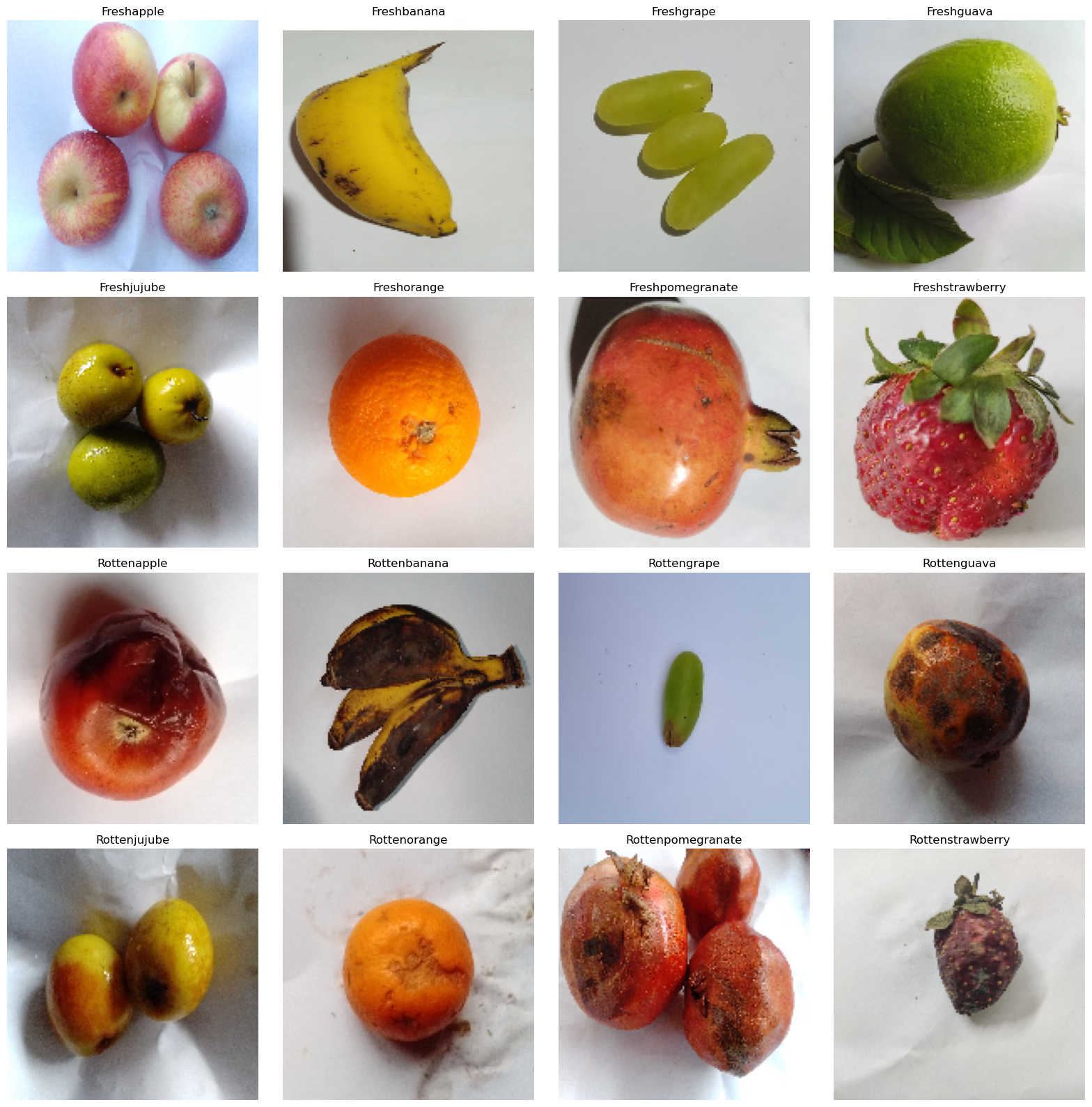
The dataset is well-balanced across the various fruit classes, which is beneficial for developing a reliable model. As we analyse images there are no further adjustments like for missing values or outliers needed. Below are some sample images from the dataset to illustrate the variety and quality of the data.
Sample pictures of fresh and rotten fruits in the dataset
4. Model Training
Model Selection and Training
We will experiment with three variations of a Convolutional Neural Network (CNN):
- Baseline Model: A simple CNN with three convolutional layers.
- Enhanced Model: A CNN with three convolutional layers, Batch Normalization layers and dropout for regularization.
- VGG16 Pretrained Model: A CNN model based on the ImageNet pretrained VGG16, customized with a final Dense layer and an Output layer.
Each model is trained and evaluated for the Original Dataset and the augmented data set. These Image datasets are split in 80% training and 20% test data used vor validation.
CNN Baseline Model
The CNN Baseline Model consists of three Convolutional Blocks each with a Convolutional Layer and a Pooling layer. The total number of parameters is 4,762,928 from which all are trainable.
The table below summarizes the parameters in each layer, the architcture is hown in Appendix 1.
| Layer Name | Param Count | Trainable Params | Non-trainable Params | |
|---|---|---|---|---|
| 0 | Conv | 448 | 448 | 0 |
| 1 | Pooling | 0 | 0 | 0 |
| 2 | Conv | 4640 | 4640 | 0 |
| 3 | Pooling | 0 | 0 | 0 |
| 4 | Conv | 18496 | 18496 | 0 |
| 5 | Pooling | 0 | 0 | 0 |
| 6 | Flatten | 0 | 0 | 0 |
| 7 | Dense | 4735232 | 4735232 | 0 |
| 8 | Output | 4112 | 4112 | 0 |
| 9 | Total | 4762928 | 4762928 | 0 |
Below you can find the results for the original and augmented Dataset after 20 Epochs of training and a batch size of 20. Both scenarios show improved performance towards the end of the epochs. No signs of overfitting can be detected. The use of the larger augmented dataset results in improved performance.
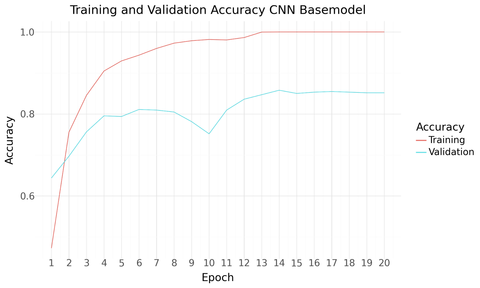
Accuracy for CNN Basemodel
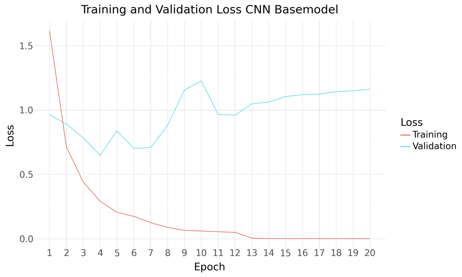
Loss for CNN Basemodel
| Accuracy | Precision | Recall | F1Score | AUC | |
|---|---|---|---|---|---|
| Epoch | |||||
| 1 | 0.643750 | 0.756813 | 0.564062 | 0.646374 | 0.965654 |
| 2 | 0.696875 | 0.787321 | 0.601562 | 0.682019 | 0.970222 |
| 3 | 0.756250 | 0.784615 | 0.717188 | 0.749388 | 0.972299 |
| 4 | 0.795313 | 0.818627 | 0.782812 | 0.800319 | 0.980803 |
| 5 | 0.793750 | 0.795455 | 0.765625 | 0.780255 | 0.970285 |
| 6 | 0.810938 | 0.821018 | 0.781250 | 0.800641 | 0.973026 |
| 7 | 0.809375 | 0.826299 | 0.795313 | 0.810510 | 0.973802 |
| 8 | 0.804688 | 0.814992 | 0.798437 | 0.806630 | 0.966704 |
| 9 | 0.781250 | 0.790143 | 0.776563 | 0.783294 | 0.956404 |
| 10 | 0.751562 | 0.768233 | 0.740625 | 0.754177 | 0.948303 |
| 11 | 0.809375 | 0.823151 | 0.800000 | 0.811410 | 0.963672 |
| 12 | 0.835938 | 0.840190 | 0.829687 | 0.834906 | 0.966890 |
| 13 | 0.846875 | 0.852381 | 0.839063 | 0.845669 | 0.964101 |
| 14 | 0.857813 | 0.858491 | 0.853125 | 0.855799 | 0.964354 |
| 15 | 0.850000 | 0.853543 | 0.846875 | 0.850196 | 0.964391 |
| 16 | 0.853125 | 0.856240 | 0.846875 | 0.851532 | 0.962202 |
| 17 | 0.854688 | 0.858491 | 0.853125 | 0.855799 | 0.961562 |
| 18 | 0.853125 | 0.855118 | 0.848437 | 0.851765 | 0.961606 |
| 19 | 0.851562 | 0.855573 | 0.851562 | 0.853563 | 0.962333 |
| 20 | 0.851562 | 0.855118 | 0.848437 | 0.851765 | 0.961671 |
| CNN Basemodel | |
|---|---|
| Epoch | 14.000000 |
| Accuracy | 0.857813 |
| Precision | 0.858491 |
| Recall | 0.853125 |
| F1Score | 0.855799 |
| AUC | 0.964354 |
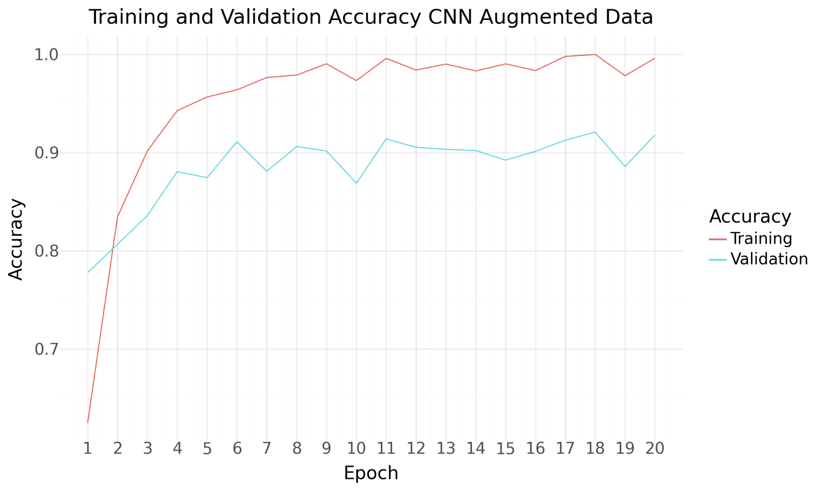
Accuracy for CNN Basemodel with Augmented Dataset
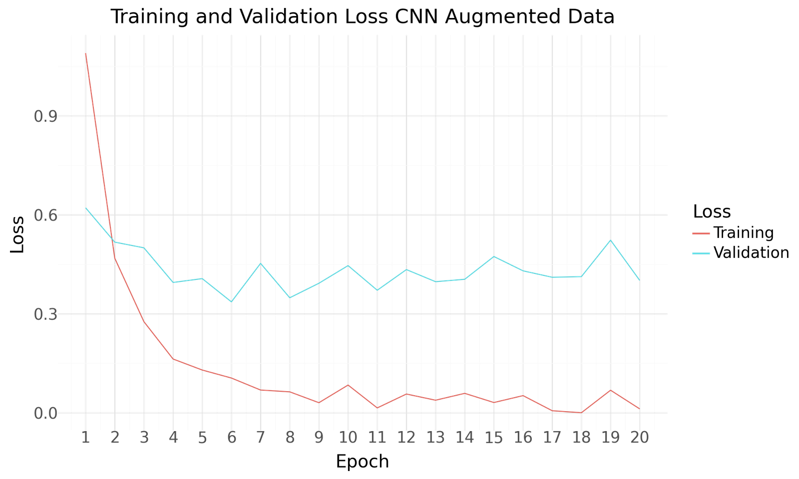
Loss for CNN Basemodel with Augmented Dataset
| Accuracy | Precision | Recall | F1Score | AUC | |
|---|---|---|---|---|---|
| Epoch | |||||
| 1 | 0.777733 | 0.826967 | 0.730191 | 0.775572 | 0.984367 |
| 2 | 0.806583 | 0.827855 | 0.777733 | 0.802011 | 0.989519 |
| 3 | 0.835839 | 0.852225 | 0.824868 | 0.838323 | 0.986587 |
| 4 | 0.880536 | 0.891205 | 0.868753 | 0.879835 | 0.988442 |
| 5 | 0.874441 | 0.884520 | 0.868346 | 0.876358 | 0.987661 |
| 6 | 0.911012 | 0.918275 | 0.908574 | 0.913399 | 0.987672 |
| 7 | 0.880943 | 0.887974 | 0.876067 | 0.881980 | 0.984029 |
| 8 | 0.906136 | 0.911632 | 0.901260 | 0.906416 | 0.989616 |
| 9 | 0.901666 | 0.907749 | 0.899634 | 0.903673 | 0.987981 |
| 10 | 0.868753 | 0.877627 | 0.865502 | 0.871522 | 0.986445 |
| 11 | 0.913856 | 0.916395 | 0.913043 | 0.914716 | 0.985344 |
| 12 | 0.905323 | 0.908497 | 0.903698 | 0.906091 | 0.984169 |
| 13 | 0.903291 | 0.908979 | 0.900853 | 0.904898 | 0.985019 |
| 14 | 0.902072 | 0.908121 | 0.899634 | 0.903858 | 0.985156 |
| 15 | 0.892320 | 0.896975 | 0.891508 | 0.894233 | 0.983038 |
| 16 | 0.901260 | 0.907005 | 0.899634 | 0.903305 | 0.982904 |
| 17 | 0.912637 | 0.915137 | 0.911418 | 0.913274 | 0.982341 |
| 18 | 0.920764 | 0.921856 | 0.920358 | 0.921106 | 0.983386 |
| 19 | 0.885819 | 0.890389 | 0.884600 | 0.887485 | 0.977844 |
| 20 | 0.917920 | 0.920343 | 0.915482 | 0.917906 | 0.984839 |
| CNN Augmented Data | |
|---|---|
| Epoch | 18.000000 |
| Accuracy | 0.920764 |
| Precision | 0.921856 |
| Recall | 0.920358 |
| F1Score | 0.921106 |
| AUC | 0.983386 |
CNN with Batch Normalization
The secon CNN Model adds Batch Normalization and Dropout layers to the Baseline Model. The total number of parameters is slightly increased to 4,764,400 from which all are trainable.
The table below summarizes the parameters in each layer, the architcture is hown in Appendix 2.
| Layer Name | Param Count | Trainable Params | Non-trainable Params | |
|---|---|---|---|---|
| 0 | conv2d | 448 | 448 | 0 |
| 1 | batch_normalization | 64 | 32 | 32 |
| 2 | max_pooling2d | 0 | 0 | 0 |
| 3 | dropout | 0 | 0 | 0 |
| 4 | conv2d_1 | 4640 | 4640 | 0 |
| 5 | batch_normalization_1 | 128 | 64 | 64 |
| 6 | max_pooling2d_1 | 0 | 0 | 0 |
| 7 | dropout_1 | 0 | 0 | 0 |
| 8 | conv2d_2 | 18496 | 18496 | 0 |
| 9 | batch_normalization_2 | 256 | 128 | 128 |
| 10 | max_pooling2d_2 | 0 | 0 | 0 |
| 11 | dropout_2 | 0 | 0 | 0 |
| 12 | flatten | 0 | 0 | 0 |
| 13 | dense | 4735232 | 4735232 | 0 |
| 14 | batch_normalization_3 | 1024 | 512 | 512 |
| 15 | dropout_3 | 0 | 0 | 0 |
| 16 | dense_1 | 4112 | 4112 | 0 |
| 17 | Total | 4764400 | 4763664 | 736 |
Below you can find the results for the original and augmented Dataset after 20 Epochs of training and a batch size of 20. Both scenarios show improved performance towards the end of the epochs. No signs of overfitting can be detected. As with the previous model the use of the larger augmented dataset results in improved performance.
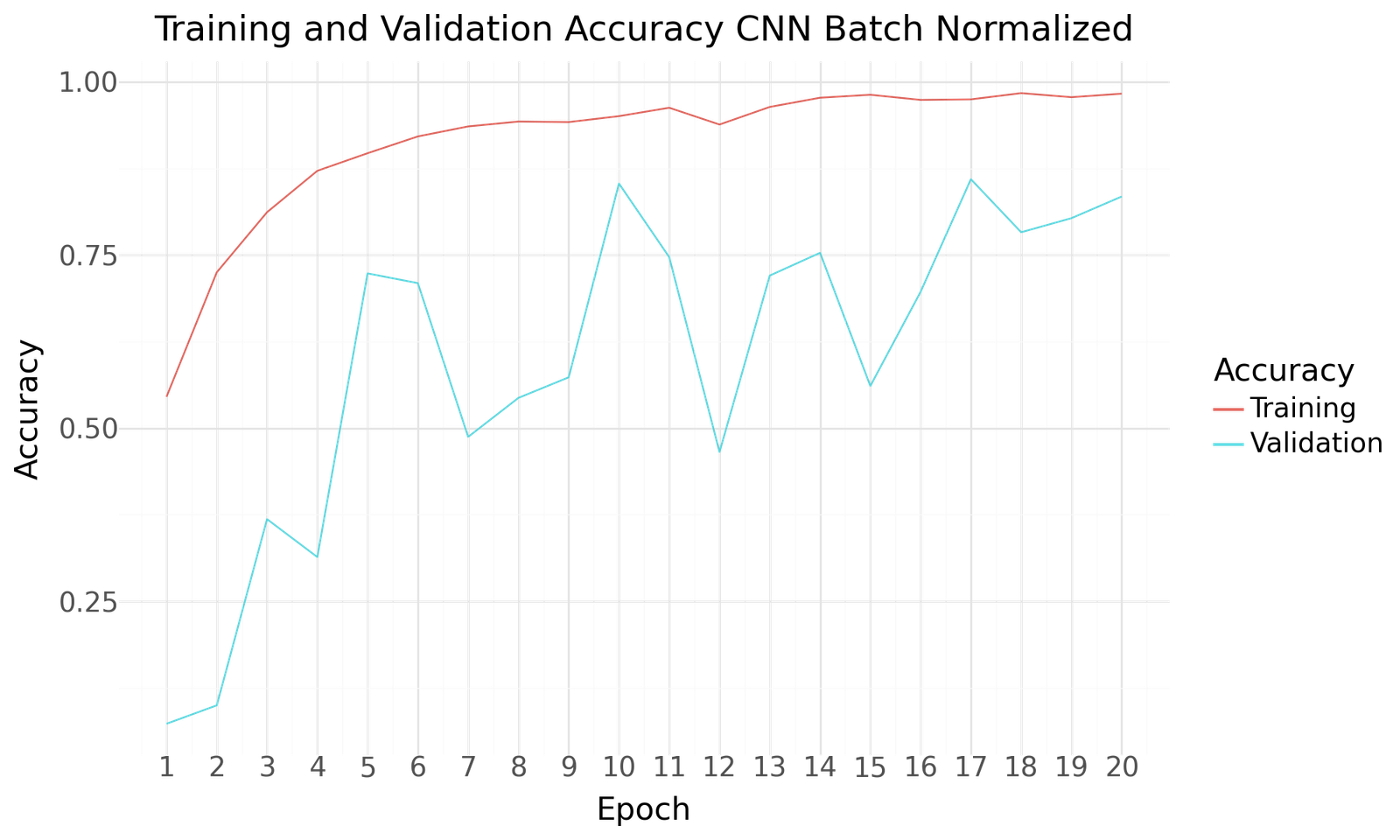
Accuracy Loss for CNN Batch Normalization
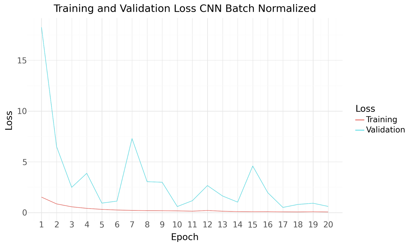
Loss for CNN Batch Normalization
| Accuracy | Precision | Recall | F1Score | AUC | |
|---|---|---|---|---|---|
| Epoch | |||||
| 1 | 0.073437 | 0.073437 | 0.073437 | 0.073437 | 0.520742 |
| 2 | 0.100000 | 0.108257 | 0.092188 | 0.099578 | 0.588592 |
| 3 | 0.368750 | 0.425358 | 0.325000 | 0.368468 | 0.840214 |
| 4 | 0.314063 | 0.336502 | 0.276563 | 0.303602 | 0.786681 |
| 5 | 0.723437 | 0.760908 | 0.681250 | 0.718879 | 0.966903 |
| 6 | 0.709375 | 0.737024 | 0.665625 | 0.699507 | 0.953470 |
| 7 | 0.487500 | 0.518707 | 0.476562 | 0.496743 | 0.819383 |
| 8 | 0.543750 | 0.592672 | 0.429688 | 0.498188 | 0.865377 |
| 9 | 0.573438 | 0.584844 | 0.554688 | 0.569366 | 0.896289 |
| 10 | 0.853125 | 0.868932 | 0.839063 | 0.853736 | 0.986776 |
| 11 | 0.746875 | 0.762684 | 0.728125 | 0.745004 | 0.959929 |
| 12 | 0.465625 | 0.497355 | 0.440625 | 0.467274 | 0.849185 |
| 13 | 0.720312 | 0.744646 | 0.706250 | 0.724940 | 0.936291 |
| 14 | 0.753125 | 0.771987 | 0.740625 | 0.755981 | 0.957774 |
| 15 | 0.560938 | 0.579565 | 0.540625 | 0.559418 | 0.848984 |
| 16 | 0.696875 | 0.710824 | 0.687500 | 0.698967 | 0.936877 |
| 17 | 0.859375 | 0.874799 | 0.851562 | 0.863025 | 0.985133 |
| 18 | 0.782812 | 0.807566 | 0.767187 | 0.786859 | 0.969630 |
| 19 | 0.803125 | 0.819063 | 0.792188 | 0.805401 | 0.962914 |
| 20 | 0.834375 | 0.855519 | 0.823438 | 0.839172 | 0.979792 |
| CNN Batch Normalized | |
|---|---|
| Epoch | 17.000000 |
| Accuracy | 0.859375 |
| Precision | 0.874799 |
| Recall | 0.851562 |
| F1Score | 0.863025 |
| AUC | 0.985133 |

Accuracy for CNN Batch Normalization with Augmented Dataset
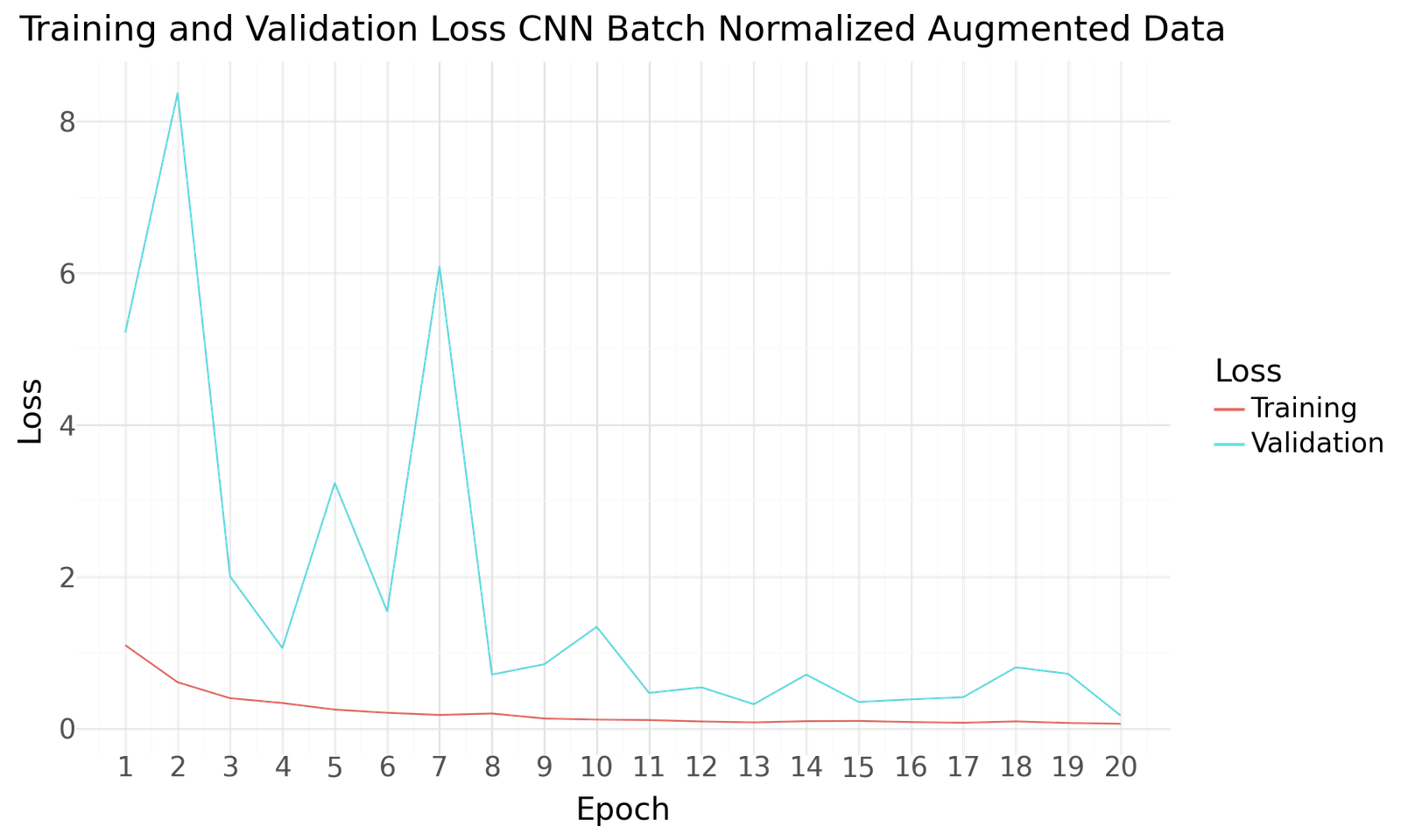
Loss for CNN Batch Normalization with Augmented Dataset
| Accuracy | Precision | Recall | F1Score | AUC | |
|---|---|---|---|---|---|
| Epoch | |||||
| 1 | 0.222674 | 0.239925 | 0.208046 | 0.222851 | 0.702998 |
| 2 | 0.460382 | 0.480301 | 0.440878 | 0.459746 | 0.793189 |
| 3 | 0.657863 | 0.691719 | 0.624543 | 0.656417 | 0.931353 |
| 4 | 0.777733 | 0.806565 | 0.748883 | 0.776654 | 0.965804 |
| 5 | 0.707030 | 0.733131 | 0.688744 | 0.710245 | 0.931503 |
| 6 | 0.789923 | 0.805731 | 0.776920 | 0.791063 | 0.956580 |
| 7 | 0.222674 | 0.241315 | 0.211703 | 0.225541 | 0.645281 |
| 8 | 0.820398 | 0.834238 | 0.811865 | 0.822900 | 0.975151 |
| 9 | 0.778952 | 0.791457 | 0.767981 | 0.779542 | 0.966592 |
| 10 | 0.706623 | 0.729149 | 0.689151 | 0.708586 | 0.938812 |
| 11 | 0.873222 | 0.889537 | 0.867127 | 0.878189 | 0.984731 |
| 12 | 0.865908 | 0.872122 | 0.861845 | 0.866953 | 0.984704 |
| 13 | 0.916701 | 0.922446 | 0.913450 | 0.917926 | 0.991996 |
| 14 | 0.826493 | 0.843384 | 0.818367 | 0.830687 | 0.972769 |
| 15 | 0.915075 | 0.921117 | 0.911012 | 0.916037 | 0.989326 |
| 16 | 0.891914 | 0.898396 | 0.887444 | 0.892886 | 0.989322 |
| 17 | 0.887850 | 0.898713 | 0.879724 | 0.889117 | 0.987485 |
| 18 | 0.811459 | 0.821473 | 0.802113 | 0.811678 | 0.971168 |
| 19 | 0.837058 | 0.847395 | 0.832588 | 0.839926 | 0.974790 |
| 20 | 0.952458 | 0.958882 | 0.947582 | 0.953198 | 0.996560 |
| CNN Batch Normalized Augmented Data | |
|---|---|
| Epoch | 20.000000 |
| Accuracy | 0.952458 |
| Precision | 0.958882 |
| Recall | 0.947582 |
| F1Score | 0.953198 |
| AUC | 0.996560 |
VGG16 Pretrained Model
The third mmodel is based on the pretrained VGG16. VGG16 is a deep convolutional neural network model that was trained on the ImageNet dataset, which contains millions of images across 1,000 classes. The model has 16 layers, including 13 convolutional layers, that are designed to extract hierarchical features from images, making it highly effective for various image classification tasks. Pretrained VGG16 on ImageNet is commonly used for transfer learning, allowing the model to be fine-tuned for specific tasks with relatively small amounts of new data. For customization we added 4 layers, a Pooling Layer, a Dense Layer an additional Dropout layer and the final Output layer. The total number of layers is 14,985,552 from which only 270,864 are trainable.
The table below summarizes the parameters in each layer, the architcture is hown in Appendix 3.
| Layer Name | Param Count | Trainable Params | Non-trainable Params | |
|---|---|---|---|---|
| 0 | input_layer_2 | 0 | 0 | 0 |
| 1 | block1_conv1 | 1792 | 0 | 1792 |
| 2 | block1_conv2 | 36928 | 0 | 36928 |
| 3 | block1_pool | 0 | 0 | 0 |
| 4 | block2_conv1 | 73856 | 0 | 73856 |
| 5 | block2_conv2 | 147584 | 0 | 147584 |
| 6 | block2_pool | 0 | 0 | 0 |
| 7 | block3_conv1 | 295168 | 0 | 295168 |
| 8 | block3_conv2 | 590080 | 0 | 590080 |
| 9 | block3_conv3 | 590080 | 0 | 590080 |
| 10 | block3_pool | 0 | 0 | 0 |
| 11 | block4_conv1 | 1180160 | 0 | 1180160 |
| 12 | block4_conv2 | 2359808 | 0 | 2359808 |
| 13 | block4_conv3 | 2359808 | 0 | 2359808 |
| 14 | block4_pool | 0 | 0 | 0 |
| 15 | block5_conv1 | 2359808 | 0 | 2359808 |
| 16 | block5_conv2 | 2359808 | 0 | 2359808 |
| 17 | block5_conv3 | 2359808 | 0 | 2359808 |
| 18 | block5_pool | 0 | 0 | 0 |
| 19 | global_average_pooling2d | 0 | 0 | 0 |
| 20 | dense_2 | 262656 | 262656 | 0 |
| 21 | dropout_4 | 0 | 0 | 0 |
| 22 | dense_3 | 8208 | 8208 | 0 |
| 23 | Total | 14985552 | 270864 | 14714688 |
Below you can find the results for the original and augmented Dataset after 20 Epochs of training and a batch size of 20. Both scenarios show improved performance towards the end of the epochs. No signs of overfitting can be detected. As with the previous two model the use of the larger augmented dataset results in improved performance.
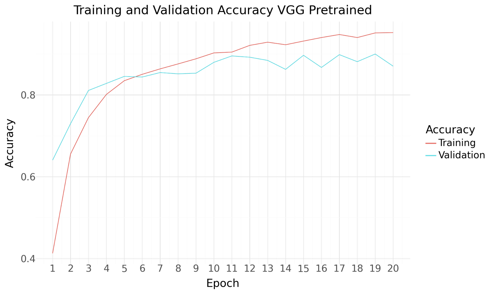
Figure 10: Accuracy for VGG Pretrained

Loss for VGG Pretrained
| Accuracy | Precision | Recall | F1Score | AUC | |
|---|---|---|---|---|---|
| Epoch | |||||
| 1 | 0.640625 | 0.878307 | 0.259375 | 0.400483 | 0.967135 |
| 2 | 0.729688 | 0.848485 | 0.481250 | 0.614158 | 0.977944 |
| 3 | 0.810938 | 0.902655 | 0.637500 | 0.747253 | 0.988430 |
| 4 | 0.828125 | 0.912525 | 0.717188 | 0.803150 | 0.991159 |
| 5 | 0.845312 | 0.908571 | 0.745313 | 0.818884 | 0.991934 |
| 6 | 0.843750 | 0.896552 | 0.771875 | 0.829555 | 0.992498 |
| 7 | 0.854688 | 0.903114 | 0.815625 | 0.857143 | 0.992099 |
| 8 | 0.851562 | 0.892734 | 0.806250 | 0.847291 | 0.993120 |
| 9 | 0.853125 | 0.887564 | 0.814062 | 0.849226 | 0.992063 |
| 10 | 0.879687 | 0.913706 | 0.843750 | 0.877336 | 0.995132 |
| 11 | 0.895312 | 0.927973 | 0.865625 | 0.895715 | 0.996097 |
| 12 | 0.892187 | 0.914430 | 0.851562 | 0.881877 | 0.994368 |
| 13 | 0.884375 | 0.905941 | 0.857813 | 0.881220 | 0.994542 |
| 14 | 0.862500 | 0.891847 | 0.837500 | 0.863819 | 0.994917 |
| 15 | 0.896875 | 0.927512 | 0.879687 | 0.902967 | 0.996260 |
| 16 | 0.867188 | 0.882068 | 0.853125 | 0.867355 | 0.994096 |
| 17 | 0.898438 | 0.912052 | 0.875000 | 0.893142 | 0.995553 |
| 18 | 0.881250 | 0.898223 | 0.868750 | 0.883241 | 0.996280 |
| 19 | 0.900000 | 0.914928 | 0.890625 | 0.902613 | 0.996317 |
| 20 | 0.870313 | 0.888889 | 0.862500 | 0.875496 | 0.995460 |
| VGG Pretrained | |
|---|---|
| Epoch | 19.000000 |
| Accuracy | 0.900000 |
| Precision | 0.914928 |
| Recall | 0.890625 |
| F1Score | 0.902613 |
| AUC | 0.996317 |
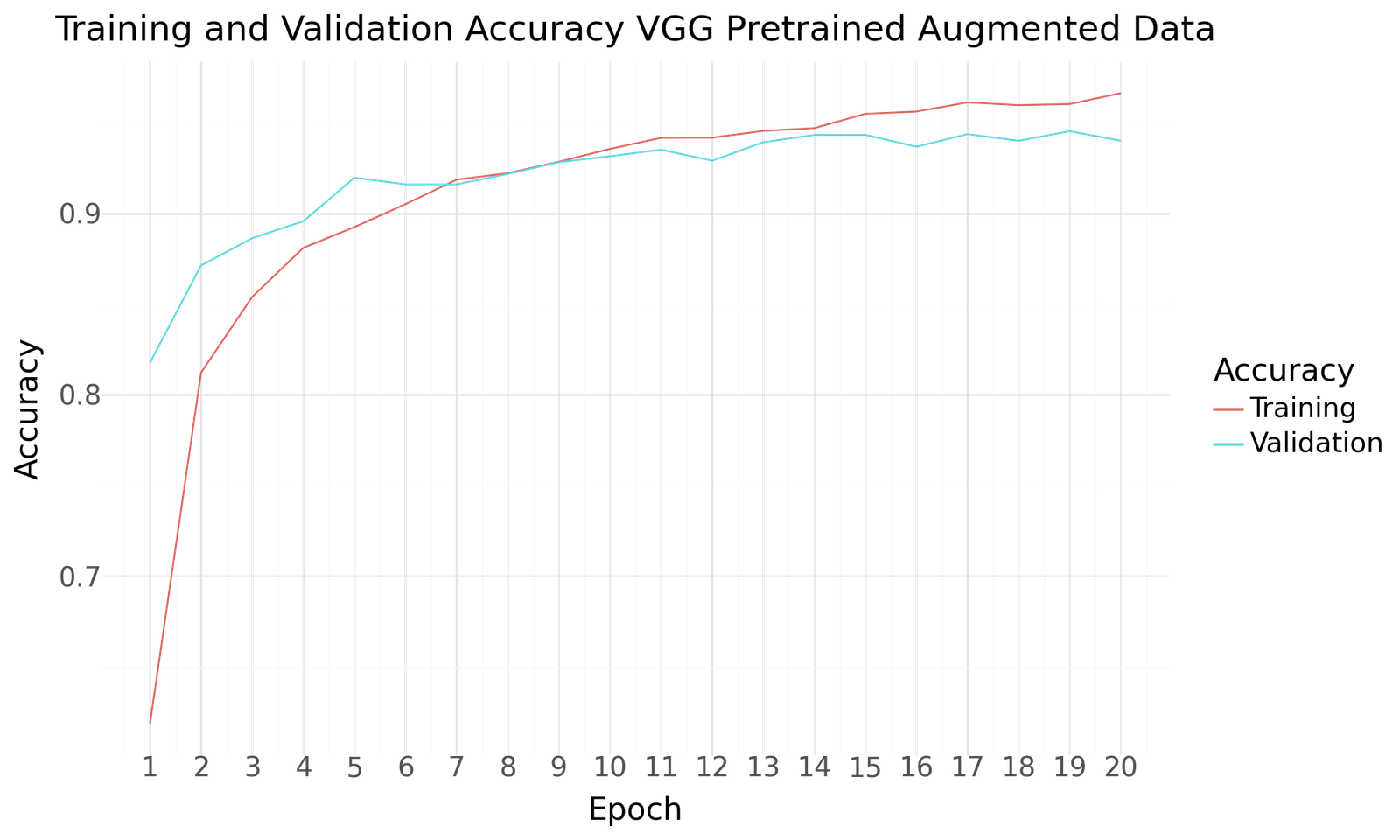
Accuracy for VGG Pretrained with Augmented Dataset
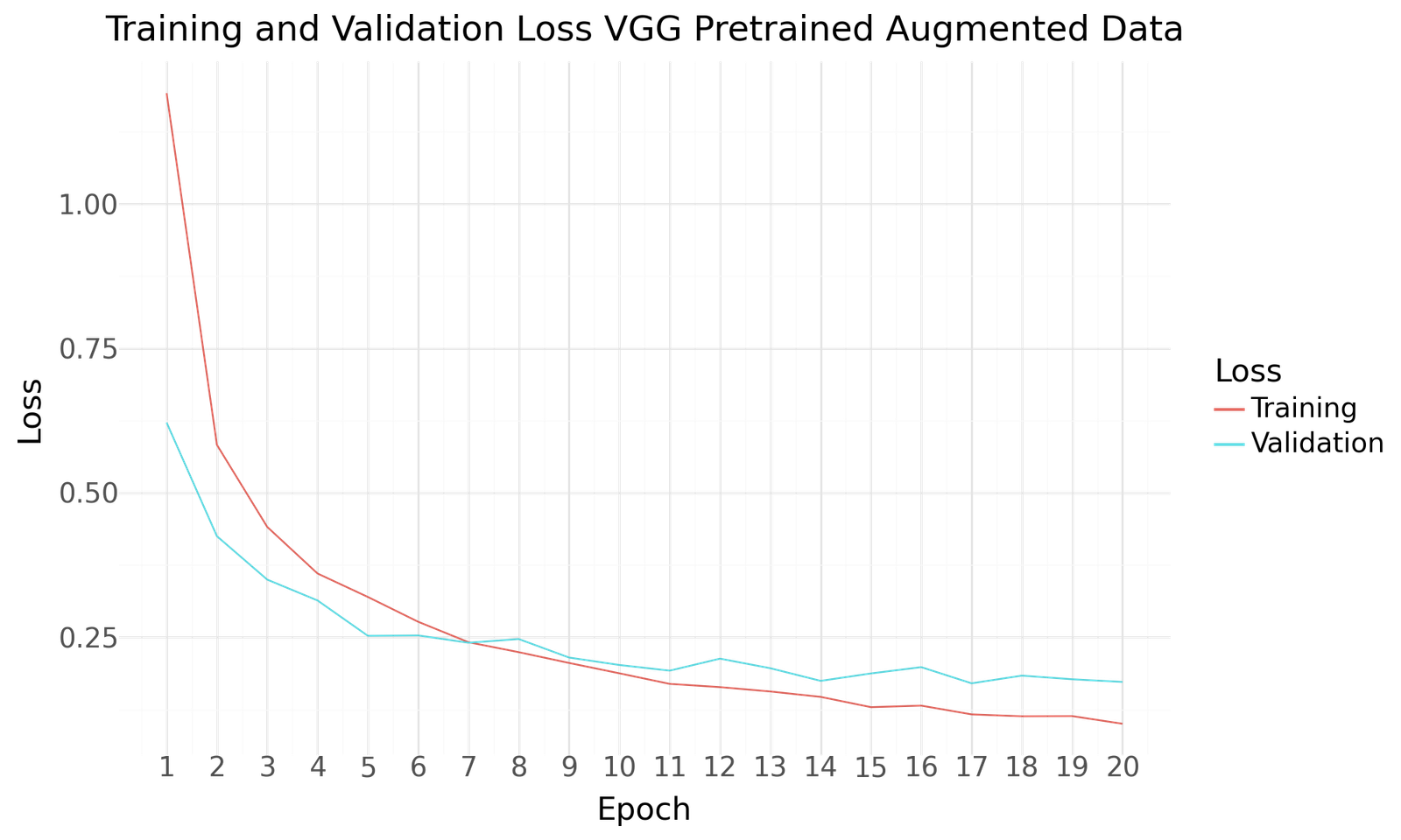
Loss for VGG Pretrained with Augmented Dataset
| Accuracy | Precision | Recall | F1Score | AUC | |
|---|---|---|---|---|---|
| Epoch | |||||
| 1 | 0.817554 | 0.920379 | 0.671678 | 0.776603 | 0.989430 |
| 2 | 0.871191 | 0.914874 | 0.812271 | 0.860525 | 0.994493 |
| 3 | 0.886225 | 0.921724 | 0.851686 | 0.885322 | 0.995999 |
| 4 | 0.895571 | 0.925315 | 0.865908 | 0.894626 | 0.996805 |
| 5 | 0.919545 | 0.938004 | 0.897603 | 0.917359 | 0.997806 |
| 6 | 0.915888 | 0.937025 | 0.900853 | 0.918583 | 0.997433 |
| 7 | 0.915888 | 0.934516 | 0.898822 | 0.916321 | 0.997447 |
| 8 | 0.921577 | 0.936762 | 0.902885 | 0.919512 | 0.997131 |
| 9 | 0.928078 | 0.941962 | 0.916701 | 0.929160 | 0.997956 |
| 10 | 0.931329 | 0.945878 | 0.923202 | 0.934403 | 0.996902 |
| 11 | 0.934986 | 0.947566 | 0.925234 | 0.936266 | 0.998272 |
| 12 | 0.928891 | 0.939469 | 0.920764 | 0.930023 | 0.996794 |
| 13 | 0.939049 | 0.947521 | 0.931735 | 0.939562 | 0.996833 |
| 14 | 0.943113 | 0.952066 | 0.936205 | 0.944069 | 0.997300 |
| 15 | 0.943113 | 0.948971 | 0.937018 | 0.942956 | 0.996994 |
| 16 | 0.936611 | 0.942387 | 0.930516 | 0.936414 | 0.996043 |
| 17 | 0.943519 | 0.950454 | 0.935392 | 0.942863 | 0.997393 |
| 18 | 0.939862 | 0.944856 | 0.932954 | 0.938867 | 0.997261 |
| 19 | 0.945144 | 0.953048 | 0.940268 | 0.946615 | 0.996702 |
| 20 | 0.939862 | 0.943535 | 0.937018 | 0.940265 | 0.997226 |
| VGG Pretrained Augmented Data | |
|---|---|
| Epoch | 19.000000 |
| Accuracy | 0.945144 |
| Precision | 0.953048 |
| Recall | 0.940268 |
| F1Score | 0.946615 |
| AUC | 0.996702 |
5. Model Evaluation and Recommendation
Model Evaluation
Each model's performance was evaluated using accuracy, precision, recall, F1 score and AUC. The table below summarizes the results:
| Epoch | Accuracy | Precision | Recall | F1Score | AUC | |
|---|---|---|---|---|---|---|
| CNN Basemodel | 14.0 | 0.857813 | 0.858491 | 0.853125 | 0.855799 | 0.964354 |
| CNN Augmented Data | 18.0 | 0.920764 | 0.921856 | 0.920358 | 0.921106 | 0.983386 |
| CNN Batch Normalized | 17.0 | 0.859375 | 0.874799 | 0.851562 | 0.863025 | 0.985133 |
| CNN Batch Normalized Augmented Data | 20.0 | 0.952458 | 0.958882 | 0.947582 | 0.953198 | 0.996560 |
| VGG Pretrained | 19.0 | 0.900000 | 0.914928 | 0.890625 | 0.902613 | 0.996317 |
| VGG Pretrained Augmented Data | 19.0 | 0.945144 | 0.953048 | 0.940268 | 0.946615 | 0.996702 |
Model Recommendation
The CNN Batch Normalized Model with Augmented Data shows the best validation accuracy and also shows great performance for all other metrics including a balance between precision and recall. This model is well-suited for the task of classifying fresh and rotten fruits.
We show the resulting confusion matrix for the augmented dataset and a validation size of 2461 images.
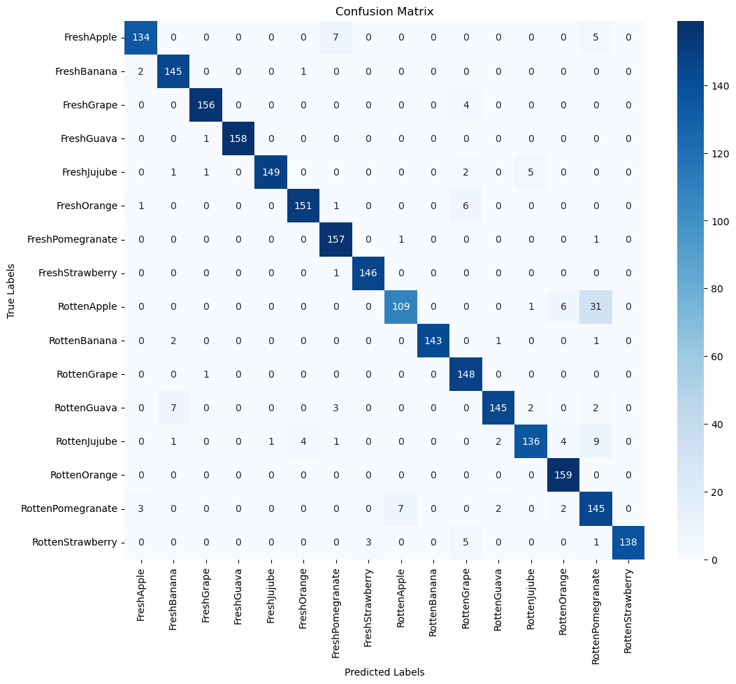
Confusion matrix for CNN Batch Normalized Model with Augmented Data
The Confusion matrix confirms the high accuracy of the model. The only outlier would be the 31 cases of Rotten Apples which were classified as Rotten Pomegranates. Rotten Oranges on the other hand were perfectly classified.
Below we present 15 examples of misclassification, one for each class of fruit (except for Rotten Oranges as mentioned without misclassification).
Examples of misclassification for CNN Batch Normalized Model with Augmented Data
We can summarize the performance for each class as shown in the Classification Report Heatmap below. Rotten Oranges have a perfect Recall value. Perfect Precision values can be found for Rotten Guavas, Rotten Bananas and Rotten Strawberries.
Classification Report for CNN Batch Normalized Model with Augmented Data
6. Key Findings and Insights
Summary of Findings
- The CNN Batch Normalized Model with Augmented Data achieved the highest accuracy of 95%, making it the most effective model for this classification task.
- Data Augmentation played a crucial role in enhancing model performance by introducing more diversity in the training data.
- The Baseline Model provided a solid starting point but was outperformed by the more complex models.
- Enhanced Model showed improved results, demonstrating the benefits of Batch Normalization architectures.
- Overall, the CNN Batch Normalized Model with Augmented Data strikes a good balance between accuracy and model complexity, making it the optimal choice for this application.
- The Pretrained VGG Model with Augmented Data shows similar performance and could be considered as alternative, while being more complex and computational intensive.
Insights
- Impact of Augmentation: The application of data augmentation techniques significantly improved the model's generalization capability, suggesting that further exploration of augmentation strategies could yield even better results.
- Model Complexity: While increasing the depth of the network improved performance, it also increased training time and computational cost, highlighting the trade-offs involved in model selection.
- Future Directions: Exploring more advanced architectures such as ResNet or using ensemble methods could potentially lead to further improvements in classification accuracy.
7. Conclusion and Next Steps
Conclusion
This analysis demonstrates the effectiveness of using a Convolutional Neural Network (CNN) for classifying fruit quality based on images. Among the models tested, the CNN Batch Normalized Model with Augmented Data stands out as the most reliable, achieving the highest accuracy and offering a balanced performance in terms of precision and recall. This model is well-suited for the task of distinguishing between fresh and rotten fruits and can serve as a robust solution for automated fruit quality assessment.
Suggestions for Future Work
- Explore Additional Data: Incorporating more fruit varieties or expanding the dataset with additional images could enhance the model’s robustness and generalizability.
- Experiment with Advanced Architectures: Testing more complex architectures such as ResNet, Inception, or DenseNet might yield further improvements in classification accuracy and model performance.
- Ensemble Methods: Investigating the use of ensemble methods, where multiple models are combined, could potentially increase the reliability of the predictions.
- Real-World Application: Consider deploying the model in a real-world setting to automate the fruit quality assessment process in retail or agricultural environments. This could involve integrating the model into an existing supply chain management system.
- Optimize for Deployment: Further work could focus on optimizing the model for deployment, including reducing its size and improving inference speed without sacrificing accuracy.
Appendix

CNN Basemodel Layers
CNN Batch Normalization Model Layers
Appendix 3:VGG Pretrained Model Layers